This week we have a guest blog post from Javier Burgués. Enjoy!
I would like to introduce you a rather unknown application of the CrazyFlie 2.0 (CF2): chemical sensing. Due to its small form-factor, the CF2 is an ideal platform for carrying out gas sensing missions in hazardous environments inaccessible to terrestrial robots and bigger drones. For example, searching for victims and hazardous gas leaks inside pockets that form within the wreckage of collapsed buildings in the aftermath of an earthquake or explosion.
To evaluate the suitability of the CF2 for these tasks, I developed a custom deck, named the MOX deck, to interface two metal oxide semiconductor (MOX) gas sensors to the CF2. Then, I performed experiments in a large indoor environment (160 m2) with a gas source placed in challenging positions for the drone, for example hidden in the ceiling of the room or inside a power outlet box. From the measurements collected in motion (i.e. without stopping) along a predefined 3D sweeping path that takes around 3 minutes, the CF2 builds a map of the gas distribution and identifies the most likely source location with high accuracy.
1. MOX deck
The MOX deck (Fig. 1a) contains two sockets for 4-pin Taguchi-type (TGS) gas sensors, a temperature/humidity sensor (SHT25, Sensirion AG), a dual-channel digital potentiometer (AD5242BRUZ1M, Analog Devices, and two MOSFET p-type transistors (NX2301P, NEXPERIA). I used TGS 8100 sensors (Figaro Engineering) due to its compatibility with 3.0 V logic, power consumption of only 15 mW (the lowest in the market as of June 2016) and miniaturized form factor (MEMS). Since the sensor heater uses 1.8V, two transistors (one per sensor) reduce the applied power by means of pulse width modulation (PWM). The MOX read-out circuit (Fig. 1b) is a voltage divider connected to the μC’s analog-to-digital converter (ADC). The voltage divider is powered at 3.0 V and the load resistor (RL) can be set dynamically by the potentiometer (from 60 Ω to 1 MΩ in steps of 3.9 kΩ). Dynamic configuration of the load resistor is important in MOX gas sensors due to the large dynamic range of the sensor resistance (several orders of magnitude) when exposed to different gas concentrations. The sensors were calibrated (by exposing them to several known concentrations) to convert the raw output into parts-per-million (ppm) concentration units.
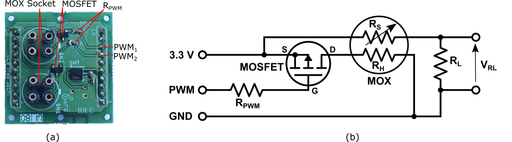
Figure 1. (a) MOX deck (without gas sensors); (b)
Schematic of the conditioning electronics for each MOX sensor.
The initialization task of the deck driver configures the PWM, initializes the SHT25 sensor, sets the wiper position of both channels of the potentiometer and adds the MOX readout registers to the list of variables that are continuously logged and transmitted to the base station. The main task of the deck driver reads the MOX sensor output voltage and the temperature/humidity values from the SHT25 and sends them to the ground station at 10 Hz.
2. Experimental Arena, External Localization System and Gas Source
Experiments were performed in a large robotics laboratory (160 m2 × 2.7 m height) at Örebro University (Sweden). The laboratory is divided into three connected areas (R1–R3) of 132 m2 and a contiguous room (R4) of 28 m2 (Fig. 2). To obtain the 3D position of the drone, I used the Loco positioning system (LPS) from Bitcraze, based on ultra-wide band (UWB) radio transmitters. Six LPS anchors were positioned in known locations of the experimental arena and one LPS tag was fixed to the drone. The six LPS anchors were placed in the central area of the laboratory, shaped in two inverted triangles (below and above the flight area).
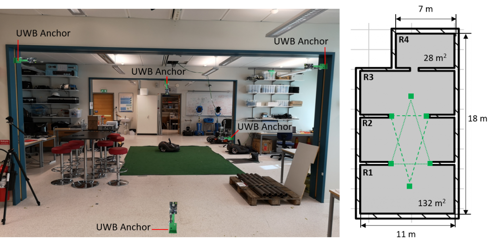
Figure 2. Experimental arena. The green squares indicate the position of the UWB anchors, which are positioned along two inverted triangles (green lines).
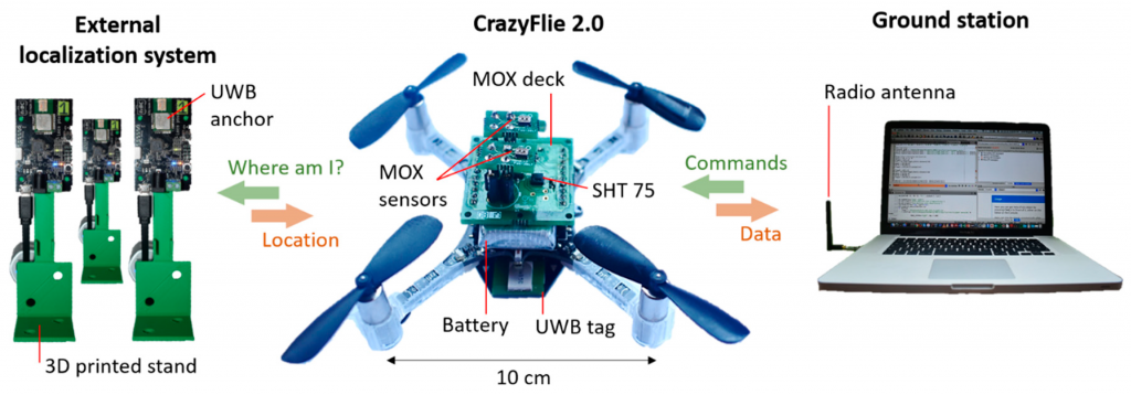
Figure 3. The CrazyFlie 2.0 equipped with the MOX deck and the UWB tag (center) gets its 3D position from the LPS system (left). The location and sensor data are communicated to the ground station (right) over the 2.4 GHz ISM band.
A gas leak was emulated by placing a small beaker filled with 200 mL of ethanol 96% in different locations of the arena (Fig. 4). Ethanol was used because it is non-toxic and easily detectable by MOX sensors. Two experiments were carried out to check the viability of the proposed system for gas source localization and mapping in complex environments. In the first experiment, the gas source was placed on top of a table (height = 1 m) in the small room (R4). In the second experiment, the source was placed inside the suspended ceiling (height = 2.7 m) near the entrance to the lab (R1). Since the piping system of the lab runs through the suspended ceiling, the gas source could represent a leak in one of the pipes. A 12 V DC fan (Model: AD0612HB-A70GL, ADDA Corp., Taiwan) was placed behind the beaker to facilitate dispersion of the chemicals in the environment, creating a plume. The experiments started five minutes after setting up the source and turning on the DC fan.
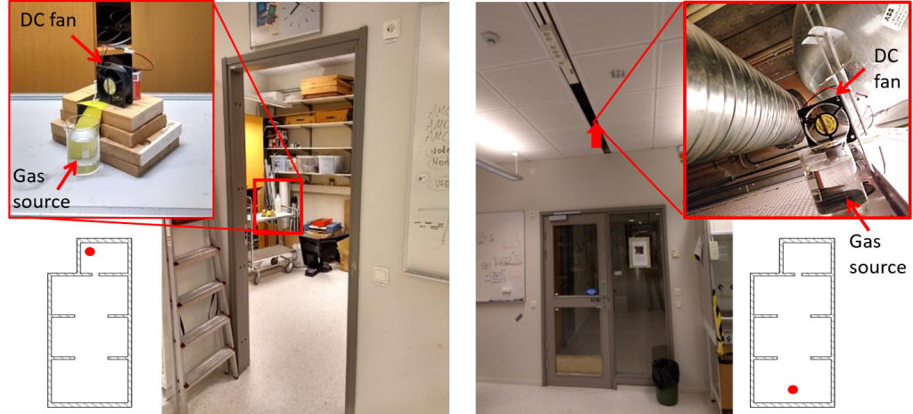
Figure 4. Gas source location in two experiments. (left) Experiment 1: inside small room; (right) Experiment 2: hidden in suspended ceiling.
3. Navigation strategy
The drone was sent to fly along a predefined sweeping path consisting of two 2D rectangular sweepings at different heights (0.9 m and 1.8 m), collecting measurements in motion (Fig. 5). These two heights divide the vertical space of the lab in three parts of equal size. Flying first at a lower altitude minimizes the impact of the propellers’ downwash in the gas distribution. For safety reasons, the trajectory was designed to ensure enough clearance around obstacles and walls, and people working inside the laboratory were told to remain in their seats during the experiments. The ground station communicates the flight path to the drone as a sequence of (x,y,z) waypoints, with a target flight speed of 1.0 m/s. The CF2 reports the measured concentration and its location to the ground station every 100 ms.
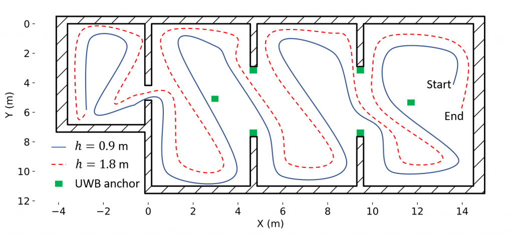
Figure 5. Predefined navigation strategy based on zig-zag sweeping at two heights (0.9 and 1.8 m).
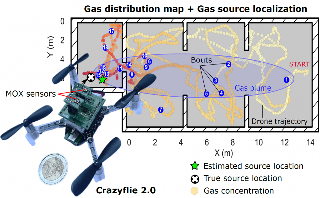
At the end of the exploration, the ground station uses all the received information to compute a 3D map of the instantaneous concentration and the ’bouts’. A ’bout’ is declared when the derivative of the sensor response exceeds a certain threshold. Bouts are produced by contact with individual gas patches and some authors use them instead of the instantaneous response (which is more affected by the slow response time of chemical sensors). For gas source localization, we compare two approaches: using the cell with maximum value in the concentration map or using the cell with maximum bout frequency. The bout frequency (bouts/min) is computed as the bout count in a 5 second sliding window multiplied by 12 (to convert it to bouts/min).
4. Results
In the first experiment, the drone took off near the entrance of the lab (R1), 17 meters downwind of a gas source located in the other end of the laboratory (R4). From the gas distribution map (Fig. 6a) it is evident that the gas source must be in R4, because the maximum concentration (35 ppm) was found there while concentrations below 5 ppm were measured in the rest of the lab. The gas plume can be outlined from the location of odor hits. The highest odor hit density (25 hits/min) was found also in R4. The cells corresponding to the maximum concentration (green start) and maximum odor hit frequency (blue triangle) were found at 0.94 and 1.16 m of the true source location, respectively.
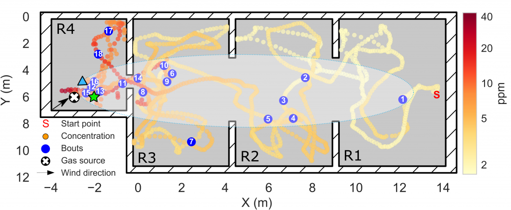
Figure 6a. 2D map of the instantaneous concentration (ppm) measured in Experiment 1 (in log scale). The odor hits are represented by blue circles. A hand-drawn ellipse outlines the approximate plume shape based on the location of odor hits.
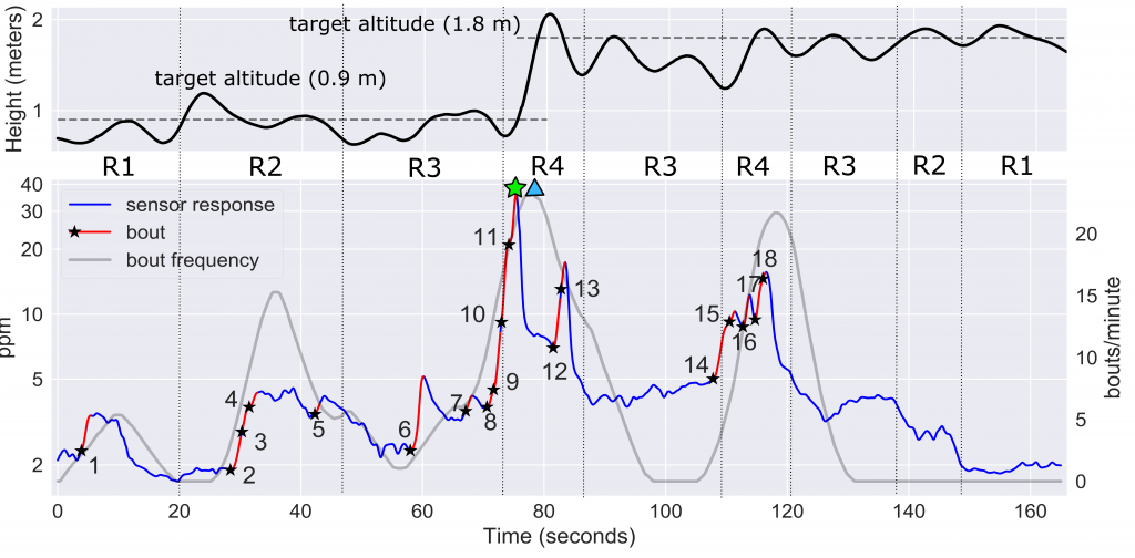
Figure 6b. (top) Trajectory of the CF2 along the z-axis. (bottom) Temporal evolution of the measured concentration (ppm) on a log scale, with odor hits highlighted in red (the black star indicates the start of an odor hit). The identifiers R1–R4 indicate the area of the map in which the drone is flying at each moment. The maximum instantaneous concentration and the maximum odor hit frequency are indicated by a green star and a blue triangle, respectively.
In the second experiment, the gas source was located just above the starting point of the exploration, hidden in the suspended ceiling (Fig. 7). The resulting maximum concentration in the test room was measured when the drone flew at h=1.8 m, highlighting the importance of sampling in 3D for localization and mapping of elevated gas sources. However, since the source is presumably not directly exposed to the environment, concentrations below 3 ppm were found in most locations of the room, which complicates the gas source localization task. The concentration and odor hit maps suggest that the gas source is located in the division between R1 and R2, which represents a localization error of 4.0 and 3.31 m, respectively.
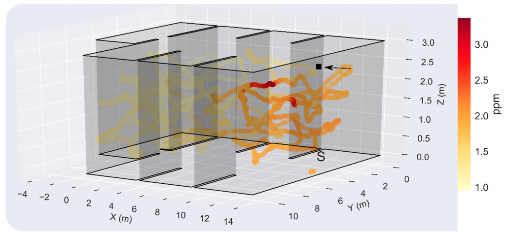
Figure 7. 3D map of the instantaneous concentration (ppm) in Experiment 2. The black square indicates the gas source location (x,y,z) = (14.0, 5.2, 2.7) m, the black arrow the wind direction (positive x-axis) and the letter ‘S’ the starting point of the drone (x,y,z) = (13.5, 5.2, 0.0) m.
5. Conclusions
These results suggest that the CF2 can be used for gas source localization and mapping in large indoor environments. In contrast to previous works in which long measurement times were taken at predefined or adaptively chosen sampling locations, a rough approximation of such maps can be obtained in very short time with concentration measurements acquired in motion. The obtained gas distribution maps seem coherent with respect to the true source location and wind direction, and not only enable the detection of the source with relatively small localization errors but also provide a rich visual interpretation of the gas distribution.
If you are interested in more details about this work, take a look at the journal paper or drop me an email at <jburgues8 at gmail dot com> or leave a comment on the blog!