We finally got some time to follow up on the previous blog post Measuring propeller RPM: Part 1. In this post we will continue where we left of and describe a little about the software we have implemented.
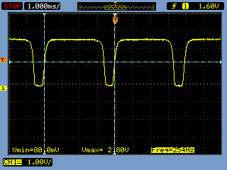 The sensor output, as showed in the scope picture, can be connected directly to a digital input. We connected them to the expansion port signals TX2, RX2, IO2 and IO3 as they are all internally connected to a timer with capture capability, TIM5_CH3, TIM5_CH4, TIM3_CH2, TIM3_CH1 respectively. With the capture functionality it is possible to trigger a timer read on events like a pin change. Thus it is not that difficult to calculate the period time of the input signal which can be used to calculate the rpm. Setting up the timer to run at 1us tick was a bit tricky but manageable. With 1us tick it will wrap around, it’s a 16 bit timer, so after 1us * 65536 = 65.5ms. This means the slowest rpm that can be measured is about 458 rpm (1/(2*65.5ms)*60). The division by 2 is because there are 2 blades on the prop. Since hovering happens way over 458 rpm it doesn’t matter much that we can’t measure any slower speed.
Next thing was to setup the capture compare. The ST library already provides the basic API, TIM_ICInitStructure, so it was more or less just a matter of finding how to configure it. The capture part of the timer can do quite fancy things but in the end we decided it was easiest to just use it the simple way, were it stores the timer value in the corresponding capture compare register on a predefined edge. As the register values will be overwritten when the next pulse comes we setup a interrupt handler to take care of the result. What the interrupt handler ended up to do was to copy the timer value, use that to calculate the rpm and then save the result in a variable. It turned out to be good to do an average of the two latest values as the pulses was not fully symmetrical because of the two blades. This was then done the same way for each propeller input and, voilà, rpm measurements was taken. (Well, there certainly was a bit of hair pulling before it all worked but in the end it worked! Love that feeling)
Getting it down to a cfclient was a piece of cake using the logging framework. We just defined the variables to be logged, setup the logging in the cfclient and it could all be plotted. The variables was defined using the macros below.
LOG_GROUP_START(rpm)
LOG_ADD(LOG_UINT16, m1, &m1rpm)
LOG_ADD(LOG_UINT16, m2, &m2rpm)
LOG_ADD(LOG_UINT16, m3, &m3rpm)
LOG_ADD(LOG_UINT16, m4, &m4rpm)
LOG_GROUP_STOP(rpm)
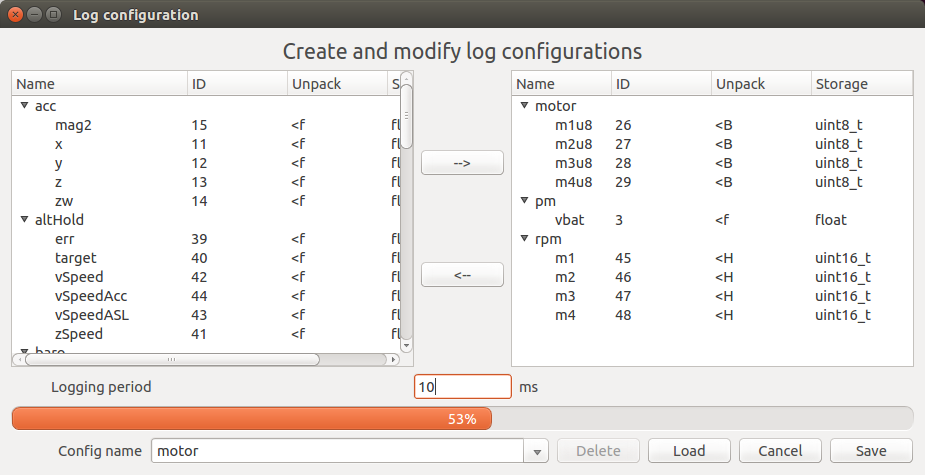
Then by connecting the the Crazyflie a log configuration could be created called “motor” containing the rpm values as well as voltage and PWM.
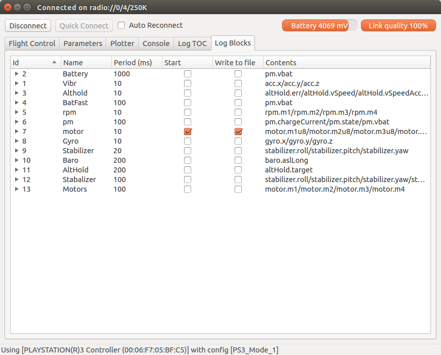
After that by opening the Log Blocks tab the “motor” log configuration could be enabled a written to files. The data log output folder can be opened from the menu by selecting “Settings -> Open config folder”. In my case in “logdata/20150202T17-29-49/motor-20150202T17-35-09.csv”. This CSV file can then be imported to a program such as Octave, Matlab, Spreadsheet etc for further analysis.
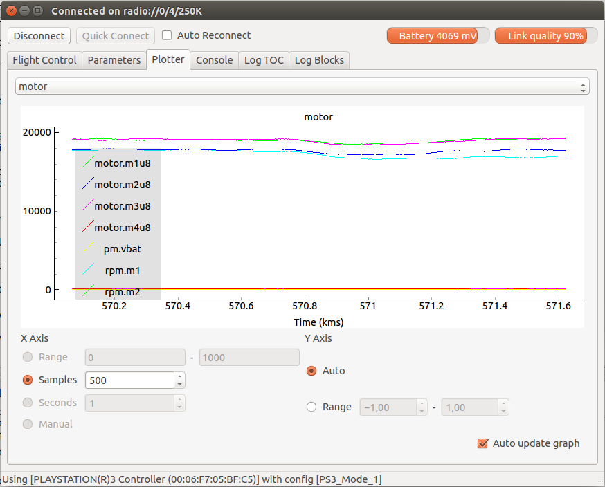
The data can also be plotted in real-time using the plotter as in the picture below. Hmmm, interesting, the Crazyflie 2.0 seems to hover at about 19000 rpm with the RPM measurement board attached.
The idea was to do the analysis part in this post as well but it turned out to be a little bit to much, therefore stay tuned for the final analyzing part!