Explaining Kalman Filters with the Crazyflie

A while ago, we wrote a generic blog post about state estimation in the Crazyflie, mostly discussing different ways the Crazyflie can determine its attitude and/or position. At that time, we only had the Complementary filter and Extended Kalman filter (EKF). Over the years, we’ve made some great additions like the M-estimation-based robust Kalman filter (an enhancement of the EKF, see this blog post) and the Unscented Kalman filter.

However, we have noticed that some of our beginning users struggle with understanding the concept of Kalman filtering, depending on whether this has been covered in their curriculum. And for some more experienced users, it might be nice to have a recap of the basics as well, since this is a very important part of the Crazyflie’s capabilities of flight (and also for robotics in general). So, in this blog post, we will explain the principles of Kalman filtering and how it is applied within the Crazyflie firmware, which hopefully will provide a good base for anyone starting to delve into state estimation within the Crazyflie.

We will also have a developer meeting about Kalman filtering on the Crazyflie, so we hope you can join that as well if you have any questions about how it all works. Also we are planning to got to FOSdem this weekend so we hope to see you there too.

Main Principles of the Kalman Filter

Anybody remotely working with autonomous systems must, at one point, have heard of the Kalman filter, as it has existed since the 60s and even played a role in the Apollo program. Understanding its main principles is also important for anyone working with drones or robotics. There are plenty of resources available, and its Wikipedia page is filled with examples, so here we will focus mostly on the concept and principles and leave the bulk of the mathematics as an exercise for those who like to delve into that :).

So basically, there are several principles that apply to a Kalman filter:

• It estimates a linear system that is driven by stochastic processes. The probability function that drives these stochastic processes should ideally be Gaussian.
• It makes use of the Bayes’ rule, which is a general term in statistics that describes the probability of an event happening based on previous knowledge related to that event.
• It assumes that the ‘to be estimated state’ can be described with a Markov model, which assumes that a sequence of the next possible event (or scenario) can be predicted by the current event. In other words, it does not need a full history of events to predict the next step(s), only the information from the event of one previous step.
• A Kalman filter is described as a recursive filter, which means that it reuses (part of) its output as input for the next filtering step.

So the state estimate is usually a vector of different variables that the developer or user of the system likes to observe, for either control or prediction, something like position and velocity, for instance: [x, y, ẋ, ẏ, …]. One can describe a dynamics model that can predict the state in the next step using only the current time step’s state, like for instance: x_t+1 = x_t + ẋ_t, y_t+1 = y_t + ẏ_t. This can also be nicely described in matrix form as well if you like linear algebra. To this model, you can also add predicted noise to make it more realistic, or the effect of the input commands to the system (like voltage to motors). We will not go into the latter in this blogpost.

The Concept of Kalman filters

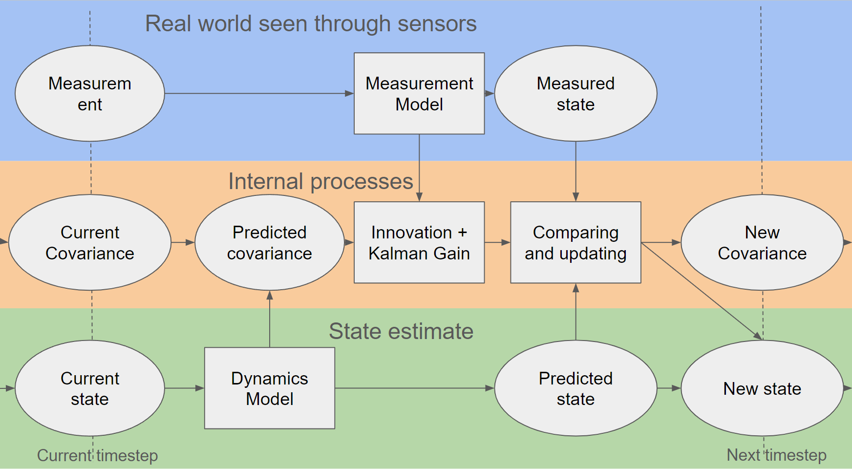
So, we will go through the process of explaining the steps of the Kalman filter now, which hopefully will be clear with the above picture. As mentioned before, we’d like to avoid formulas and are oversimplifying some parts to make it as clear as possible (hopefully…).

First, there is the predict phase, where the current state (estimate) and a dynamics model (also known as the state transition model) result in a predicted state. Also in the same phase, the predicted estimated covariance is calculated, which also uses the dynamics model plus an indication of the process noise model, indicating how much the dynamics model deviates from reality in predicting that state. In an ideal world and with an ideal model, this could be enough; however, no dynamics model is perfect, which is why the next phase is also very important.

Then it’s the update phase, where the filter estimate gets updated by a measurement of the real world through sensors. The measurement needs to go through a measurement model, which transforms the measurement into a measured state (also known as innovation or measurement pre-fit residual). Usually, a measurement is not a 1-1 depiction of one variable of the state, so the measurement model ensures that the measurement can properly be compared to the predicted state. This same measurement model, accompanied by the measurement noise model (which indicates how much the measurement differs from the real world), together with the predicted covariance, is used to calculate the innovation and Kalman gain.

The last part of the update phase is where the predictions are updated with the innovation. The Kalman gain is then used to update the predicted state to a new estimated state with the measured state. The same Kalman gain is also used to update the covariance, which can be used for the next time step.

An 1D example, height estimation

It’s always good to show the filter in some form of example, so let’s show you a simple one in terms of height estimation to demonstrate its implications.

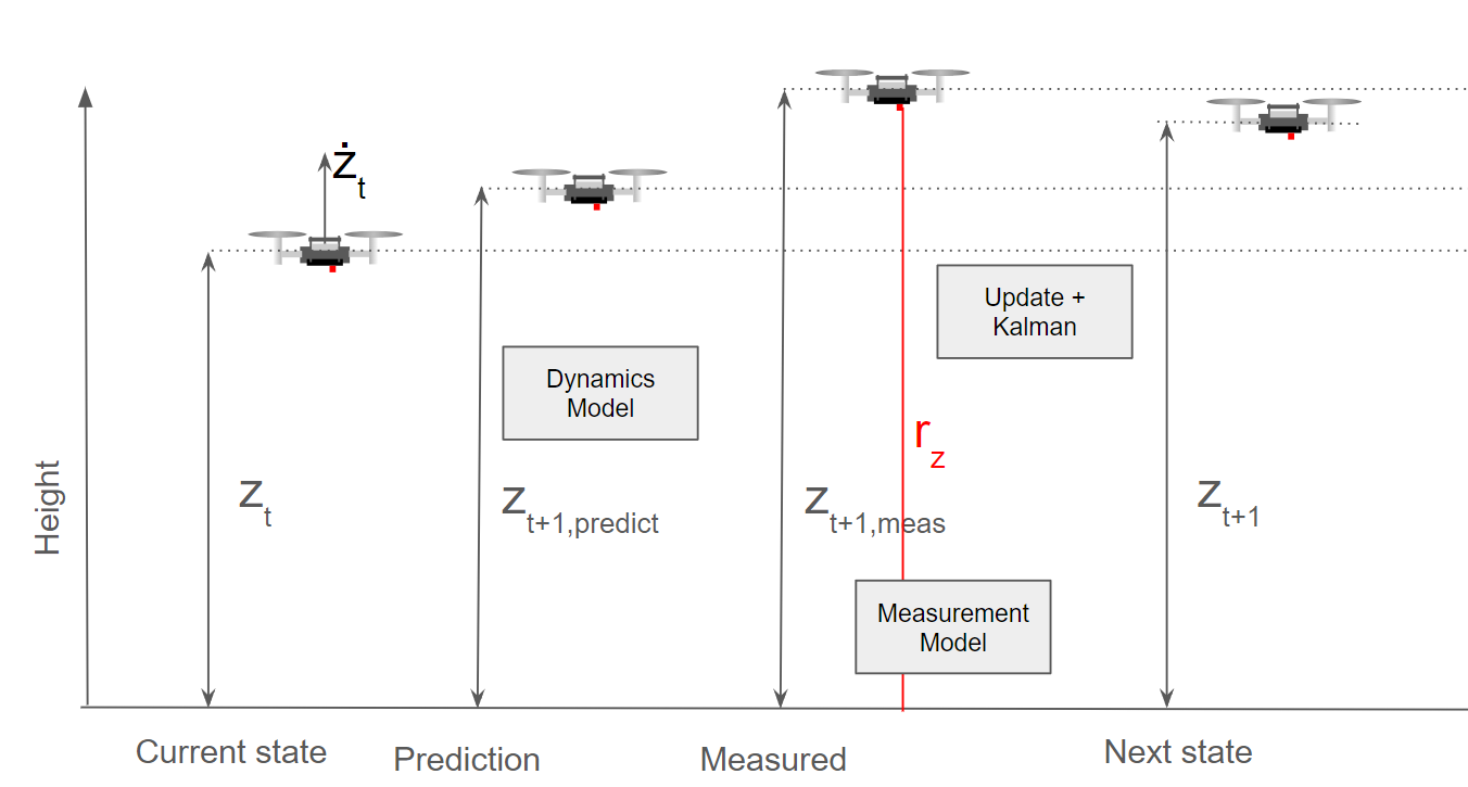
You see here a Crazyflie flying, and currently it has its height estimated at z_t and its velocity at ż_t. It goes to the predict phase and predicts the next height to be at z_t+1,predict, which is a simple model of just z_t + ż_t. Then for the innovation and updating phase, a measurement (from a range sensor) r_z is used for the filter, which is translated to z_{t+1, meas}. In this case, the measurement model is very simple when flying over a flat surface, as it probably is only a translation addition of the sensor to the middle of the Crazyflie, or perhaps a compensation for a roll or pitch rotation.

In the background, the covariances are updated and the Kalman gain is calculated, and based on z_t+1,predict and z_{t+1, meas}, the next state z_t+1 is calculated. As you probably noticed, there was a discrepancy between the predicted height and measured height, which could be due to the fact that the dynamics model couldn’t correctly predict the height. Perhaps a PID gain was higher than expected or the Crazyflie had upgraded motors that made it climb faster on takeoff. As you can see here, the filter put the estimated height closer to z_t+1 to the measurement than the predicted height. The measurement noise model incorporated into the covariances indicates that the height sensor is more accurate than the height coming from the dynamics model. This would very well be the case for an infrared height sensor like the one on the Flow Deck; however, if it were an ultrasound-based sensor or barometer instead (which are much noisier), then the predicted height would be closer to the one predicted by the dynamics model.

Also, it’s good to note that the dynamics model does not currently include the motor input, but it could have done so as well. In that case, it would have been better able to predict the jump it missed now.

A 2D example, horizontal position

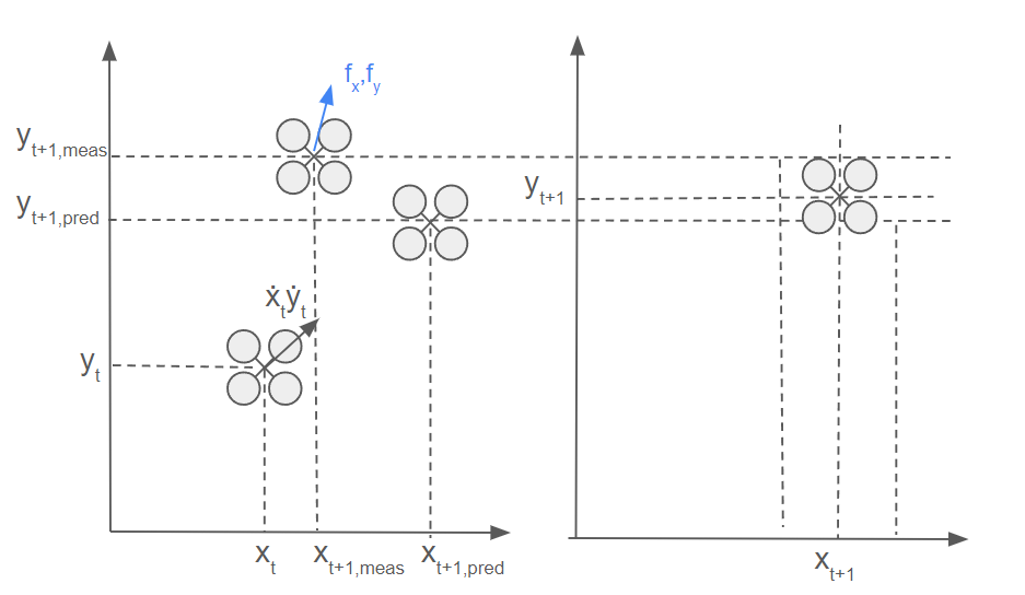
Let’s take it up a notch and add an extra dimension. You see here now that there is a 2D solution of the Crazyflie moving horizontally. It is at position x_t, y_t and has a velocity of ẋ_t, ẏ_t at that moment in time. The dynamics model estimates the Crazyflie to end up in the general direction of the velocity factor, so it is a simple addition of the current position and velocity vector. If the Crazyflie has a flow sensor (like on the Flow Deck), flow f_x, f_y can be detected and translated by the measurement model to a measured velocity (part of the state filter) by combining it with a height measurement and camera characteristics.

However, the measurement in the form of the measured flow f_x, f_y estimates that there is much more flow detected in the x-direction than in the y-direction. This can be due to a sudden wind gust in the y-direction, which the dynamics model couldn’t accurately predict, or the fact that there weren’t as many features on the surface in the y-direction, making it more difficult for the flow sensor to measure the flow in that direction. Since this is not something that both models can account for, the filter will, based on the Kalman gain and covariances, put the estimate somewhere in between. However, this is of course dependent on the estimated covariances of both the outcome of the measurement and dynamic models.

In case of non-linearity

It would be much simpler if the world’s processes could be described with linear systems and have Gaussian distributions. However, the world is complex, so that is rarely the case. We can make parts of the world more abstract in simulation, and Kalman filters can handle that, but when dealing with real flying vehicles, such as the Crazyflie, which is considered a highly nonlinear system, it needs to be described by a nonlinear dynamics model. Additionally, the measurements of sensors in more complex and 3D situations usually don’t have a one-to-one linear relationship with the variables in the state. Can you still use the Kalman filter then, considering the earlier mentioned principles?

Luckily certain assumptions can be made that can still make Kalman filters useful in the sense of non-linearity.

• Extended Kalman Filter (EKF): If there is non-linearity in either the dynamics model, measurement models or both, at each prediction and update step, these models are linearized around the current state variables by calculating the Jacobian, which is a collection of first-order partial derivative calculations of the model and the state variables.
• Unscented Kalman Filter (UKF): An unscented Kalman filter deals with linearities by selecting sigma points selected around the mean of the state estimate, which are backpropagated through the non-linear dynamics model.

However, there is also the case of non-Gaussian processes in both dynamics and measurements, and in that case a complementary filter or particle filter would be best suited. The Crazyflie contains a complementary filter (which does not estimate x and y), an extended Kalman filter and an experimental unscented Kalman filter. Check out the state-estimation documentation for more information.

So…. where is the code?

This is all fine and dandy, however… where can you find all of this in the code of the Crazyflie firmware? Here is an overview of where you can find it exactly in the sense of the most used filter of them all, namely the Extended Kalman Filter.

• Initialize the state and variances kalmanCoreInit() in kalman_core.c
• Prediction step with the dynamics model: predictDt() in kalman_core.c
• Innovation and update of the covariance with the measurement update: kalmanCoreScalarUpdate() in kalman_core.c
  • All measurement models can be found in seperate files in the kalman_core/ folder
  • The height measurement model for TOF range sensor like in the 1D example: kalmanCoreUpdatewithToF() in mm_tof.c
  • The flow measurement model for the flow sensor like in the 2D example: kalmanCoreUpdateWithFlow() in mm_flow.c
• Finalizing the state (by rotating all the state variables in the correct orientation: kalmanCoreFinalize() in kalman_core.c

There are several assumptions made and adjustments made to the regular EKF implementation to make it suitable for flight on the Crazyflie. For those details I’d like to refer to the papers on where this implementation is based on, which can be found in the EKF documentation. Also for a more precise explanation of Kalman filter, please check out the lecture slides of Stanford University on Linear dynamical systems or the Linköping university’s course slides on Sensor Fusion.

Update: From the comments we also got notified of an nice EKF tutorial where you write the filter from scratch (github) from Prof. Simon D. Levy from Washington and Lee university. Practice makes perfect!

Next Developer meeting and FOSdem

As you would have guessed, our next developer meeting will be about the Kalman filters in the Crazyflie. Keep an eye on this Discussion thread for more details on the meeting.

Also Kimberly and Arnaud will be attending FOSdem this weekend in Brussels, Belgium. We are hoping to organize an open-source robotics BOF/meetup there, so please let us know if you are planning to go as well!