State Estimation

Today we will have a guest blogpost by Dominik Natter, working in the Robotics & Control group at SINTEF in Trondheim, Norway. Enjoy!!

In this blogpost we will teach you how to fly the Crazyflie beyond edges without crashing, using only on-board sensors. Come join in!

flying over edges — Safe flights across edges are achievable!

Introduction

UAVs have seen tremendous progress in the last decades and have since moved from research labs to various real-world environments. Small UAVs (so-called micro air vehicles, MAVs) like the Crazyflie open up even more possibilities. For example, their size allows them to traverse narrow passages or fly in cluttered environments (as recently showcased in this blog post). However, in order to achieve these complex tasks the community must further improve the cognitive ability of these MAVs in order to avoid crashes.

One task on this list and today’s topic is the possibility to fly at constant altitude irrespective of the terrain. This feature has been discussed in the community already two years ago. To understand the problem, let’s look at the currently implemented solution: With the Flow deck mounted the Crazyflie uses a 1D lidar sensor to estimate its vertical position. This vertical position (more or less) equals the current sensor reading. On flat floors this solution works very well. However, if the Crazyflie shall traverse through a narrow window or fly above irregular terrain its altitude will change based on the sensor readings. This can lead to unstable flights, as in the following video, or even crashes!

You might wonder: why not use any of the other great tools from the Bitcraze universe? Indeed, the Lighthouse positioning system and the Loco positioning system work well for absolute positioning (as we have seen earlier, e.g., in this blog post). However, the required setups are often not available in difficult environments. Alternatively, the barometer could be used to achieve a solution based solely on on-board sensors. In fact, Bitcraze has proposed an altitude hold functionality a few years ago. This is a cool feature, but its positioning accuracy of “roughly ±15cm” is not fully satisfying. Finally, relying on the on-board IMU alone will inevitably lead to drifting over time.

Thus, we propose a solution based on the Flow deck and the Multiranger deck. This approach, only based on on-board sensors, allows to fly at constant altitude with obstacles above, below, or even both above and below the Crazyflie. Kristoffer Skare developed this solution when he worked with us as an intern in 2021.

Technical Description

As a first step, the upward-facing lidar of the Multiranger deck is incorporated in the same way the downward-facing lidar of the Flow deck is used in the firmware. This additional measurement can then be used in the extended Kalman filter (EKF) to improve the state estimation. Currently, the EKF estimates and outputs 1 value for the altitude. For our purpose two more states are added to the EKF: one state is defined as the height of the object under the Crazyflie compared to the height where the altitude state is defined as 0. Similarly, the other state is defined as the height of the object above the Crazyflie compared to the same reference height. The Crazyflie keeps therefore track of the environment in order to keep its own altitude constant. To achieve this, an edge detection was implemented: The errors between the predicted and measured distance are tracked in both the upward or downward range measurement. If either of these errors is too large the algorithm assumes that the floor or roof has changed (while the original EKF would think the drone’s position has changed, triggering a change in thrust). Thus, the corresponding state gets updated. For more details on the technical implementation and the code itself, check out our pull request.

Results

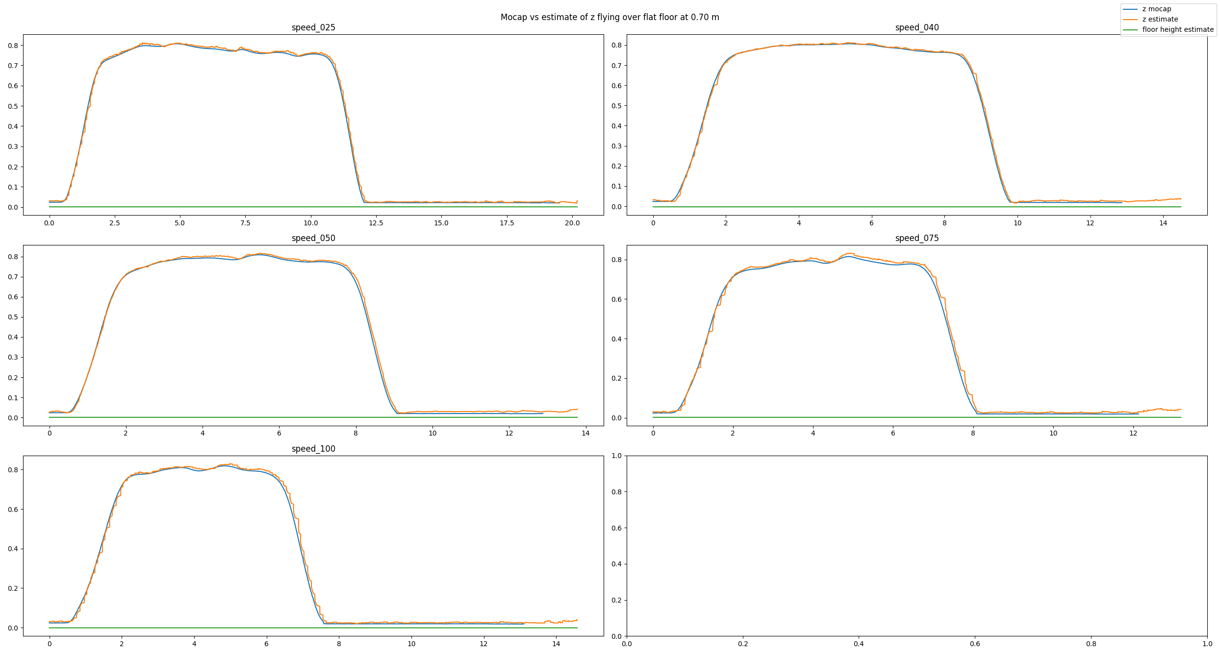
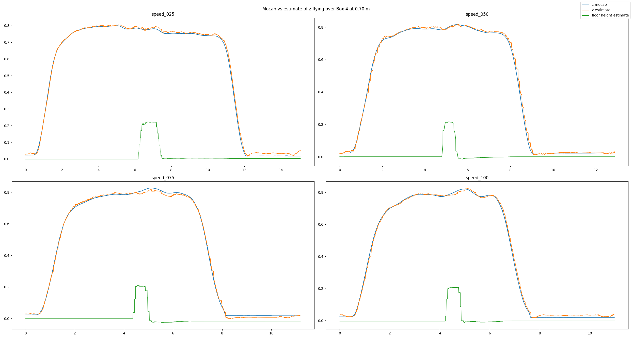
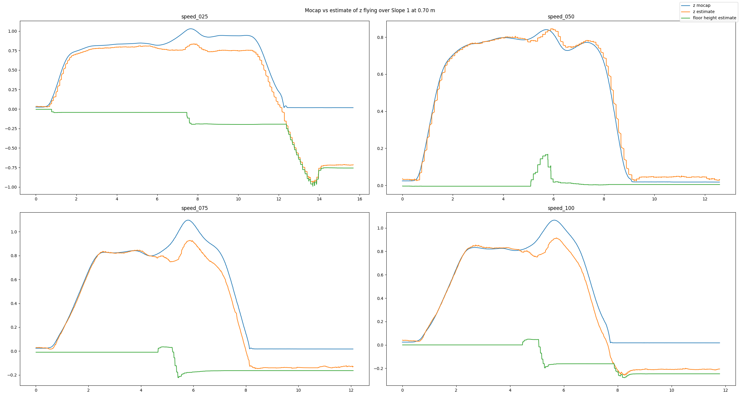
To analyze our approach we have used a Qualisys motion capture system. We have conducted many different tests: flying over different obstacles, flying at different velocities, flying at different altitudes, or even flying under different lighting conditions. Exemplarily, in this post we will have a look at a baseline example, a good estimate, and a bad estimate. In each picture you can see the altitude (in meters) over time (in seconds) for different flight speeds (in centimeters per second). You will see three lines: The motion capture ground truth (blue), the altitude estimated by our code (orange), and the new state keeping track of the floor height (green). For each plot, the Crazyflie takes off, flies in positive x direction, and lands.

In the baseline experiment, it flies over a flat floor. Clearly, the altitude estimates follow the ground truth values well, and the floor is correctly estimated to be flat.

In the next example, we have added a box with an approximate height of 0.225 m and made the Crazyflie fly over it. Despite the obstacle the altitude estimates follow the ground truth values well. Note how the floor estimates indicates the shape of the box.

experiment with box — Experiment flying over a box

Because the algorithm is based on an edge detection, we had a hunch that smoothly changing obstacles will pose a problem. Indeed, the estimates can be messy as we see in the next example. Here, the Crazyflie flies over an orthogonal triangle, with the short leg at 0.23 m pointing upwards and the long leg with 0.65 m pointing in flight direction (thus forming a slope). For different flight speeds different the estimates turn out quite differently.

experiment with slope — Experiment flying over a slope

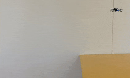
If you don’t like looking at plots, check out this video with some cool shots instead!

Conclusion

To summarize, we propose a solution for constant altitude flight with Crazyflies, using the Flow deck and the Multiranger deck. We have tested it successfully under various circumstances. Still, we see some potential for improvement, e.g. when dealing with slopes. In addition, the current implementation is quite a change to the original EKF, which poses a problem for integration.

Thus, a way forward can be an out-of-tree build to ease the use of the solution for the community. At SINTEF we certainly plan to deploy this code in all of our tests in 2022, which will hopefully allow us to gather more experience and thus find further ways to improve or tune the system.

We want to emphasize that this is not a perfect solution. That means a) you should use it with care and b) you are very much welcomed to contribute. E.g. feel free to chime in in the pull request, test the code in your environments, propose improvements, or implement an out-of-tree build! :) Maybe you can even come up with an alternative approach for constant altitude flights?

If you want to check out more of our work, visit our website. Also, keep reading this amazing blog from Bitcraze as we try to be back some day (if Bitcraze wants us hehe)!

Accurate indoor localization is a crucial enabling technology for many robotic applications, from warehouse management to monitoring tasks. Ultra-wideband (UWB) localization technology, in particular, has been shown to provide robust, high-resolution, and obstacle-penetrating ranging measurements. Nonetheless, UWB measurements are still corrupted by non-line-of-sight (NLOS) communication and spatially-varying biases due to doughnut-shaped antenna radiation pattern. In our recent work, we present a lightweight, two-step measurement correction method to improve the performance of both TWR and TDoA-based UWB localization. We integrate our method into the Extended Kalman Filter (EKF) onboard a Crazyflie and demonstrate a closed-loop position estimation performance with ~20cm root-mean-square (RMS) error.

A stylized depiction of our UWB indoor localization system and the schematics of the proposed estimation framework.

Methodology

UWB measurement errors can be separated into two groups: (1) systematic bias caused by limitations in the UWB antenna pattern and (2) spurious measurements due to NLOS and multi-path propagation. We propose a two-step UWB bias correction approach exploiting machine learning (to address(1)) and statistical testing (to address (2)). The data-driven nature of our approach makes it agnostic to the origin of the measurement errors it corrects.

(1) Neural Network Bias Correction

The doughnut-shaped antenna radiation pattern causes the relative poses of anchors and tags to have a noticeable impact on the received signal power, which leads to systematic, predictable biases. To empirically demonstrate the systematic measurement errors resulting from varying the relative pose between anchors and tags, we placed two DWM1000 UWB anchors at a distance of 4m and collected both TWR and TDoA UWB range measurements for the UWB tag mounted on top of a Crazyflie spinning around its own z-axis.

Left: schematics of the ranges (∆p’s), azimuth (α’s) and elevation angles (β’s) defining the relative poses of tag T and anchors A₀, A₁ when collecting the systematic bias measurements. Right: the neural network’s inferred bias (in red) with respect to the tag’s varying azimuth angle towards anchor T₀, α_T0, plotted against the UWB raw measurements.

We choose to leverage the nonlinear representation power of neural networks to learn the systematic bias which only depends on anchor-tag relative poses. Considering the limited onboard computation power, we select a fully connected neural network with 50 neurons in each of two layers with ReLU activation. To represent the relative pose between the UWB tag and anchors, we select the relative distance ∆p and roll, pitch, and yaw angles of the quadcopter as the input features x for the network. As we used fixed anchors, we do not include their poses as inputs (this level of generalization is left for future work). Given sufficient training data, the spatially-varying measurement bias can be described by a nonlinear function b=f(x) captured by the trained neural network.

(2) Outlier (Spurious Measurements) Rejection

Besides our learning-based bias correction, we use a quadcopter’s dynamic model to filter inconsistent UWB range measurements. Given the estimated velocity v and maximum acceleration a_max, we can compute the maximum distance d_max a quadcopter can cover during time ∆t. Based on this information, we can reject unattainable measurements before fusing them into the EKF by comparing the measurement innovation with d_max.

Moreover, we use a statistical hypothesis test to further classify potential outlier measurements. Since the measurement innovation vector is assumed to be distributed according to a multivariate Gaussian distribution, the normalized sum of squares of its values should follow a Chi-square distribution. We use the Chi-square hypothesis test to determine whether a measurement innovation is likely coming from this distribution.

UWB measurement bias f (x) prediction performance of the trained neural network (in red) compared to the actual measurement errors (blue dots) as well as the role of model-based filtering (purple dots) and statistical validation (orange dots) in rejecting outlier measurement innovations (teal dots) during a 60” flight experiment.

Data Collection and Training

We use a Crazyflie 2.0 quadcopter and the Loco Positioning System (LPS)’s UWB DW1000 modules as our research platforms. Our calibration approach runs on the Crazyflie STM32 microcontroller within the FreeRTOS real-time operating system. We equipped a cuboid flying arena with 8 UWB anchors, one for each vertex. The anchor positions were measured using a Leica total station theodolite.

Left: three-dimensional plot of our flight arena showing the positions and poses of the eight UWB DW1000 anchors (each facing towards its own x-axis, i.e., the red versor). Right: two of the training trajectories we flew to collect the samples that we used to train our neural network-based bias estimator

For all experiments, the ground truth position of the Crazyflie was provided by 10 Vicon cameras. The neural network was trained using PyTorch. To perform inference on the Crazyflie’s microcontroller, we re-use PyTorch’s trained weights in a plain C re-implementation. Since the DW1000 modules in the LPS provide UWB measurements every 5ms, the neural network inference runs at 200Hz during flight as well. Our outlier rejection method is also implemented in plain C and merged with the onboard EKF.

Close-loop Position Estimation Performance

We demonstrate the position estimation and close-loop performance of the proposed methods by flying a Crazyflie quadcopter along planar and non-planar circular trajectories (which were not among the trajectories used for training). A comparison between the estimation error of (A) the UWB localization estimate enhanced with outlier rejections and (B) the estimated enhanced with both outlier rejection and neural network bias compensation is conducted in our experiments for both TWR and TDoA2 modes. We repeated all of our experiments 10 times with a target velocity of 0.375m/s. The quadcopter trajectories during these flight tests are displayed in the following plots.

Flight paths and the tracking performance of our approach with (in blue) and without (in orange) the neural network bias correction for two reference trajectories (planar and non-planar circular orbits) and both UWB modes (TWR and TDoA).

The distributions of the RMS estimation errors are summarized into a box plot. TWR-based ranging results in better localization performance than TDoA. However, we observe that, with our neural network bias compensation, the average RMS error of TDoA localization is around 0.21m, which is comparable to that of TWR-based localization (~0.19m). Thanks to the neural network bias compensation, the average reduction in the RMS error is ~18.5% and 48% for TWR and TDoA, respectively. Most notably, this result suggests that bias compensation might help closing the performance gap between TWR- and TDoA-based localization.

Root mean square error (RMSE) of the quadcopter position estimate before (in orange) and after (in blue) the neural network calibration step for both TWR and TDoA ranging modes. Each pair of box plots refers to a planar reference trajectory (left of each pair) and a reference trajectory with varying z (right of each pair), showing a greater performance enhancement for the latter.

Outlook

In this work, we presented a two-step methodology to improve UWB localization—for both TWR- and TDoA-based measurements. We used a lightweight neural network to model and compensate for pose-dependent and spatially-varying biases and an outlier rejection mechanism to filter spurious measurements. Through several real world flight experiments tracking different trajectories, we showed that we are able to improve localization accuracy for both TWR and TDoA, granting safer indoor flight. In our future work, we will include the anchors’ pose information to allow our method to further generalize to previously unobserved indoor environments, with different anchor configurations.

Links

The authors are with the Dynamic Systems Lab, Institute for Aerospace Studies, University of Toronto, Canada, and affiliated with the Vector Institute for Artificial Intelligence in Toronto.

Feel free to contact us if you have any questions or ideas: wenda.zhao@robotics.utias.utoronto.ca. Please cite this as:

<code>@article{wenda2020learning,
  title={Learning-based Bias Correction for Ultra-wideband Localization of Resource-constrained Mobile Robots},
  author={Wenda Zhao and Abhishek Goudar and Jacopo Panerati and Angela P. Schoellig},
  journal={arXiv preprint arXiv:2003.09371},
  year={2020}
}</code>

A Modified EKF for Constant Altitude Flights