This week we have a guest blog post from Anirudha Majumdar from Mechanical & Aerospace Engineering, Princeton University. Enjoy !
Overview
The course “Introduction to Robotics” at Princeton (MAE 345 / ECE 345 / COS 346) introduces students to fundamental theoretical and algorithmic principles in robotics. We use the Crazyflies to bring the excitement of drones to students in their very first introductory course in robotics. The course is primarily aimed at undergraduate students in their third and fourth years, and also offers a graduate-level track. In Fall 2021, approximately seventy undergraduate students and ten graduate students enrolled in the course from a variety of different majors: Mechanical and Aerospace Engineering, Computer Science, Electrical and Computer Engineering, Mathematics, Operations Research and Financial Engineering, Civil and Environmental Engineering, and Architecture.
The course covers the following technical topics:
Feedback Control;
Motion Planning;
State estimation, localization, and mapping;
Computer vision and learning;
Broader topics: Robotics and the law, ethics, and economics.
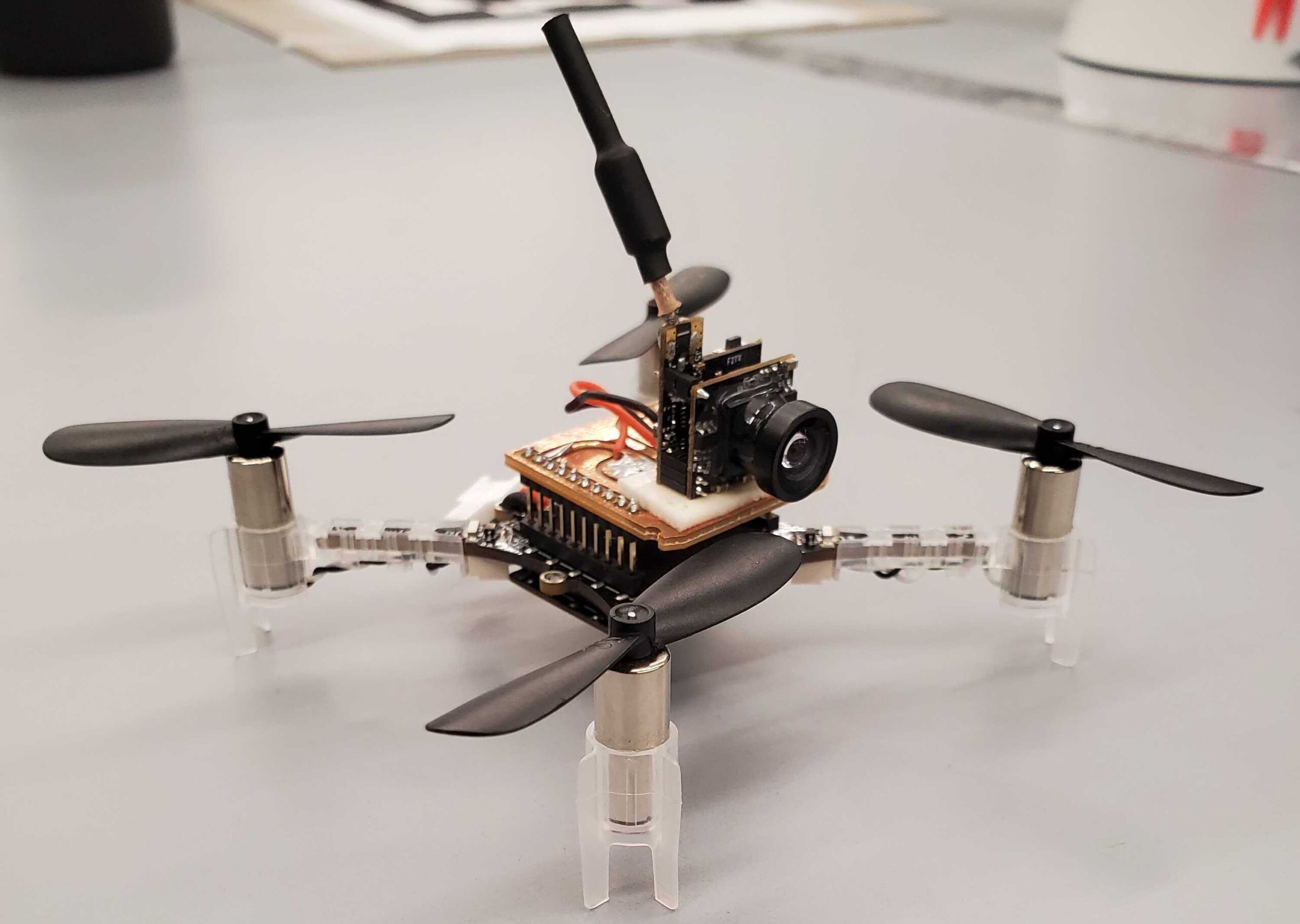
One of the primary aims of the course is to allow students to obtain hands-on experience implementing various algorithms on a hardware platform. For this, we use the Crazyflie 2.1 quadrotors with a camera attachment (Fig. 1). The Crazyflie is an ideal hardware platform for our course due to its light weight, reliability, safety, and open-source code. Throughout the semester, students work in teams to implement different algorithms from the course:
(i) linear quadratic regulator (LQR) for stabilizing the drone
(ii) rapidly-exploring randomized trees (RRTs) for motion planning through a forest of PVC pipe obstacles
(iii) the Lucas-Kanade optical flow algorithm
(iv) object-following with neural networks.
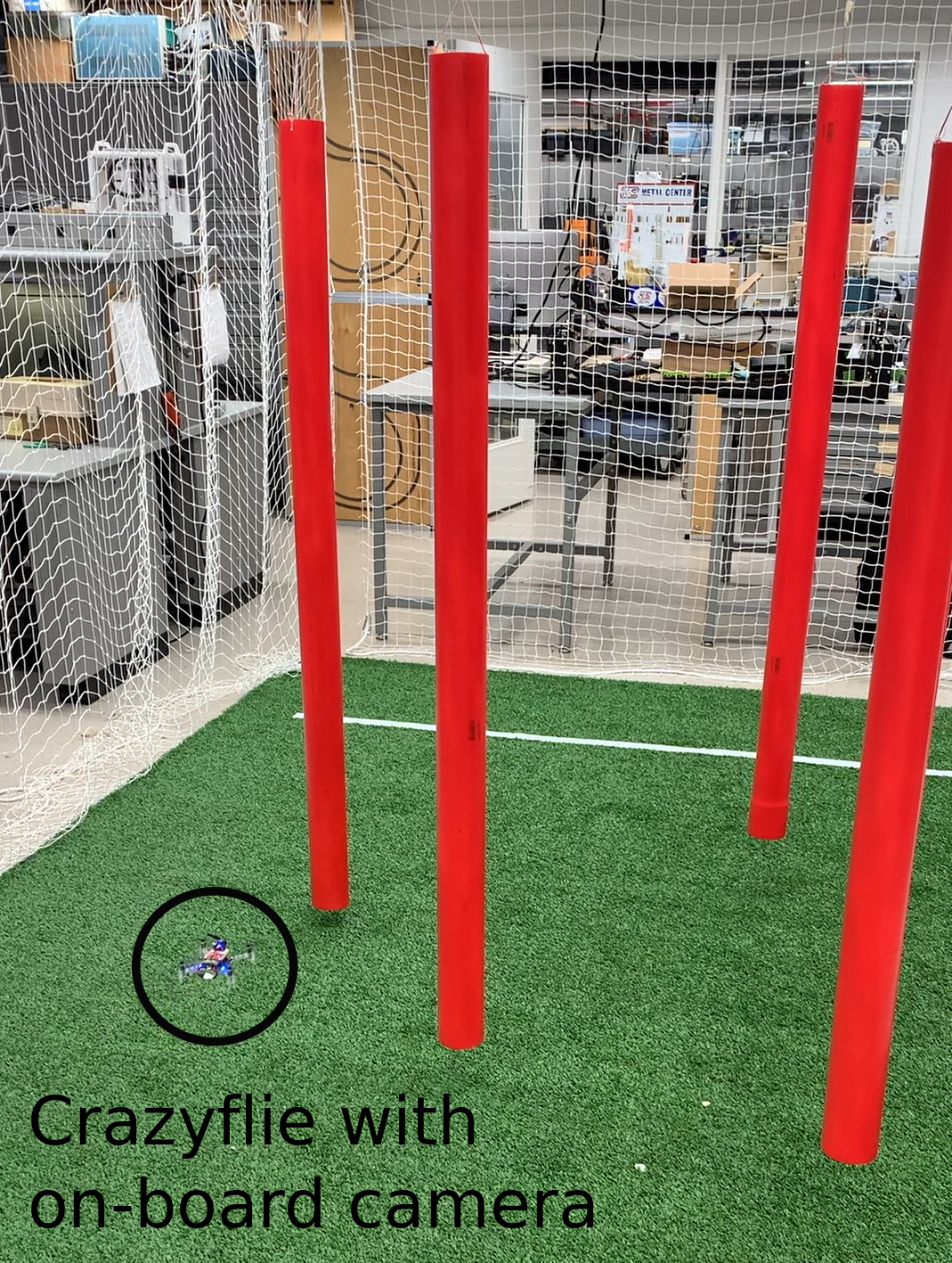
In the final project, students implement algorithms for autonomous vision-based navigation through novel (i.e., a prioriunknown) obstacle environments (Fig. 2). Below, we describe the modified Crazyflies used for the course, along with the hands-on projects in more detail.
Open-source course materials and website
We have made the course materials (lecture notes, slides, and assignments) freely available through our course website. The assignments include theory questions, programming assignments in Python, and hardware implementation with the Crazyflie. All programming and hardware assignments are freely-available through GitHub. We hope that the course materials will be useful to instructors at other institutions in getting the next generation of engineers excited about robotics!
Fig. 1. Crazyflie with a camera attachment.
Fig. 2. Vision-based navigation.
Final project for course: vision-based navigation and target-seeking.
Hardware components and lab spaces
The feedback control and motion planning hardware assignments can be completed with the following parts list:
For the vision-based assignments, we attach cameras to the drones, which transmit images in real-time to a receiver unit plugged into to a laptop. This requires the following additional parts:
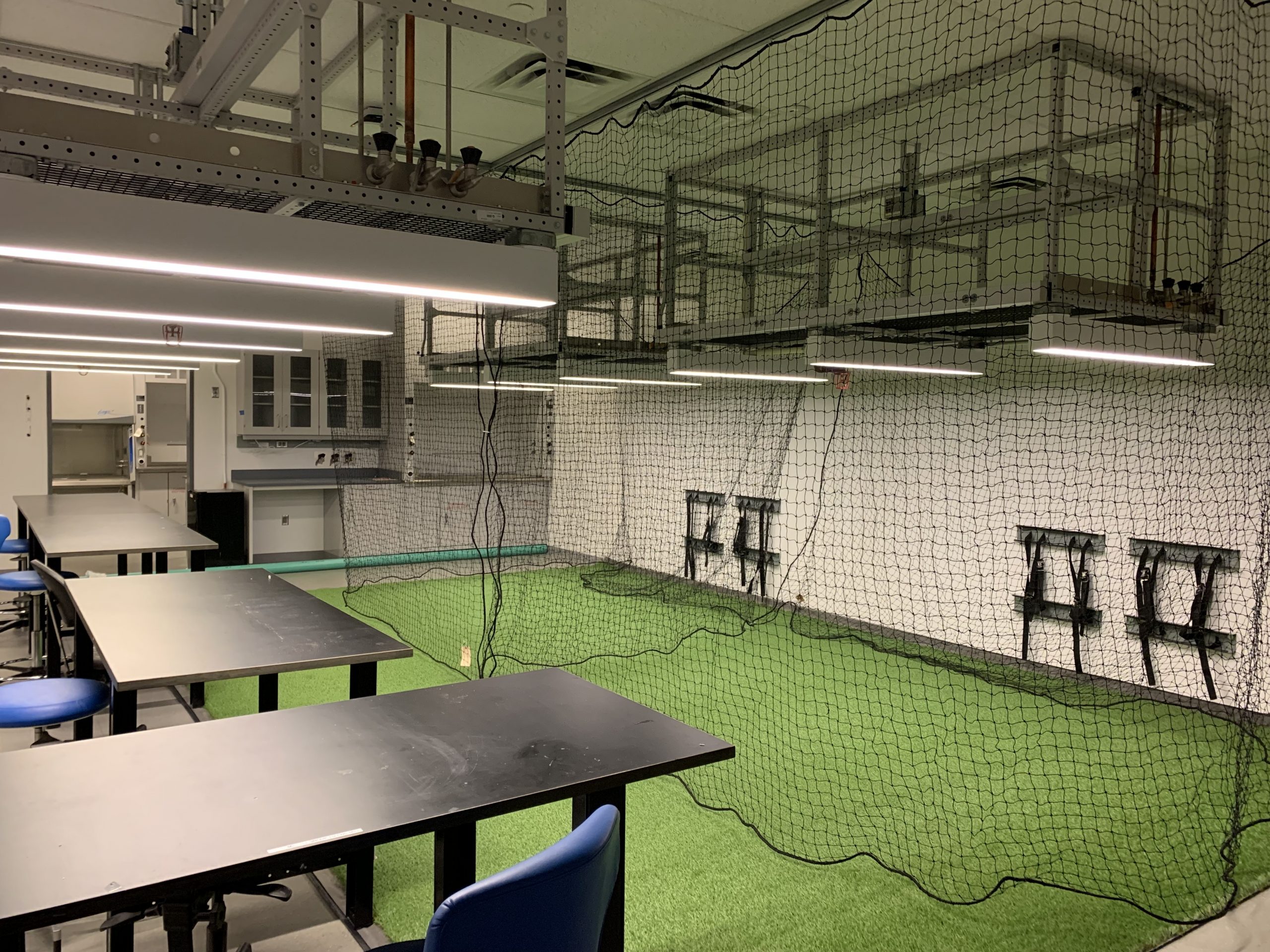
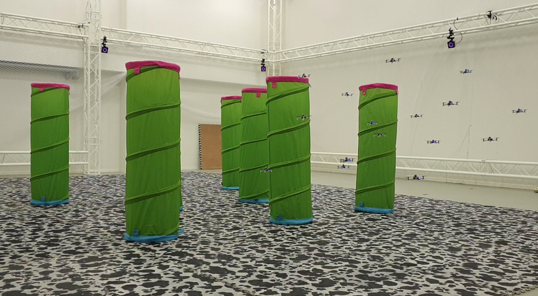
We set up three netted arenas for students to complete hardware assignments. Each arena is approximately 12 ft x 8 ft in size; two of the arenas are shown in Fig. 3.
Fig. 3. Two netted flying arenas used for the course.
Crazyflie assignments
Lab 1: Linear Quadratic Regulator (LQR)
In the first hardware lab, students implement and tune a Linear Quadratic Regulator (LQR) controller to make the drone hover. This builds on the theoretical foundations of feedback control covered in the first module of the course. Implementing LQR control on a physical system allows students to get a sense for the “reality gap”, i.e., assumptions made by the theory that are not perfectly satisfied in real life (e.g., linear dynamics, perfect state estimation, and perfect knowledge of the dynamics). This assignment makes use of a modified version of the Crazyflie firmware that allows us to upload different controller gains (obtained using LQR) and run these on the drones. Code for this assignment is available here.
Lab 2: Rapidly-Exploring Randomized Trees (RRTs)
In the second lab, students implement the RRT algorithm for motion planning. Each netted arena is set up with PVC pipe obstacles (similar to Fig. 2). Students measure the obstacle locations and radii and use the RRT algorithm to find a collision-free path from a starting location to a goal location. The Crazyflie then uses its waypoint tracking capabilities to execute the motion plan. Code for this assignment is available here.
Lab 3: Lucas-Kanade optical flow
In the computer vision module of the course, we first introduce students to “classical” vision approaches (before discussing modern deep learning techniques). One of the primary algorithms we discuss in this module is the Lucas-Kanade algorithm for computing optical flow (which has many applications such as computing time-to-collision). Students record a video using the drone’s on-board camera attachment and process this offline to compute optical flow. Code for this assignment is available here.
Lab 4: Object tracking
In the computer vision module of the course, we introduce students to deep learning-based approaches to vision. As a demonstration of the power of deep learning, we use neural networks to perform real-time object detection. Specifically, students use neural networks trained on the Coco dataset to detect a person (or an object such as a cup) using the drone’s camera, and use the resulting bounding box to command the drone in a way that makes it follow the person or object. The neural networks can be run on standard laptop computers at >= 30Hz, allowing the drone to follow the person or object in real-time. Code for this assignment is available here.
Final project: Vision-based obstacle avoidance and target-seeking
In the final project for the course, students implement vision-based navigation and target-seeking using the Crazyflie drones. Teams must program the drones to autonomously navigate through a forest of PVC pipes, whose locations are not known beforehand. Students utilize different computer vision algorithms (e.g., edge detection, contour finding, etc.) to detect obstacles and program strategies to avoid these obstacles. The goal is to navigate to the other side of the flying arena and land in front of a target object (in the form of a book). Again, teams use different approaches (e.g., neural networks) to find the book and then land in front of it. Further details and starter code for the project can be found here. See above for a video.
Acknowledgements
The following teaching staff have contributed greatly to the development of the materials for this course: Vincent Pacelli, Julienne LaChance, Jon Prevost, Alec Farid, Meghan Booker, Lena Rosendahl, David Snyder, Allen Ren, and Eric Lepowsky.
In this blogpost we will teach you how to fly the Crazyflie beyond edges without crashing, using only on-board sensors. Come join in!
Safe flights across edges are achievable!
Introduction
UAVs have seen tremendous progress in the last decades and have since moved from research labs to various real-world environments. Small UAVs (so-called micro air vehicles, MAVs) like the Crazyflie open up even more possibilities. For example, their size allows them to traverse narrow passages or fly in cluttered environments (as recently showcased in this blog post). However, in order to achieve these complex tasks the community must further improve the cognitive ability of these MAVs in order to avoid crashes.
One task on this list and today’s topic is the possibility to fly at constant altitude irrespective of the terrain. This feature has been discussed in the community already two years ago. To understand the problem, let’s look at the currently implemented solution: With the Flow deck mounted the Crazyflie uses a 1D lidar sensor to estimate its vertical position. This vertical position (more or less) equals the current sensor reading. On flat floors this solution works very well. However, if the Crazyflie shall traverse through a narrow window or fly above irregular terrain its altitude will change based on the sensor readings. This can lead to unstable flights, as in the following video, or even crashes!
You might wonder: why not use any of the other great tools from the Bitcraze universe? Indeed, the Lighthouse positioning system and the Loco positioning system work well for absolute positioning (as we have seen earlier, e.g., in this blog post). However, the required setups are often not available in difficult environments. Alternatively, the barometer could be used to achieve a solution based solely on on-board sensors. In fact, Bitcraze has proposed an altitude hold functionality a few years ago. This is a cool feature, but its positioning accuracy of “roughly ±15cm” is not fully satisfying. Finally, relying on the on-board IMU alone will inevitably lead to drifting over time.
Thus, we propose a solution based on the Flow deck and the Multiranger deck. This approach, only based on on-board sensors, allows to fly at constant altitude with obstacles above, below, or even both above and below the Crazyflie. Kristoffer Skare developed this solution when he worked with us as an intern in 2021.
Technical Description
As a first step, the upward-facing lidar of the Multiranger deck is incorporated in the same way the downward-facing lidar of the Flow deck is used in the firmware. This additional measurement can then be used in the extended Kalman filter (EKF) to improve the state estimation. Currently, the EKF estimates and outputs 1 value for the altitude. For our purpose two more states are added to the EKF: one state is defined as the height of the object under the Crazyflie compared to the height where the altitude state is defined as 0. Similarly, the other state is defined as the height of the object above the Crazyflie compared to the same reference height. The Crazyflie keeps therefore track of the environment in order to keep its own altitude constant. To achieve this, an edge detection was implemented: The errors between the predicted and measured distance are tracked in both the upward or downward range measurement. If either of these errors is too large the algorithm assumes that the floor or roof has changed (while the original EKF would think the drone’s position has changed, triggering a change in thrust). Thus, the corresponding state gets updated. For more details on the technical implementation and the code itself, check out our pull request.
Results
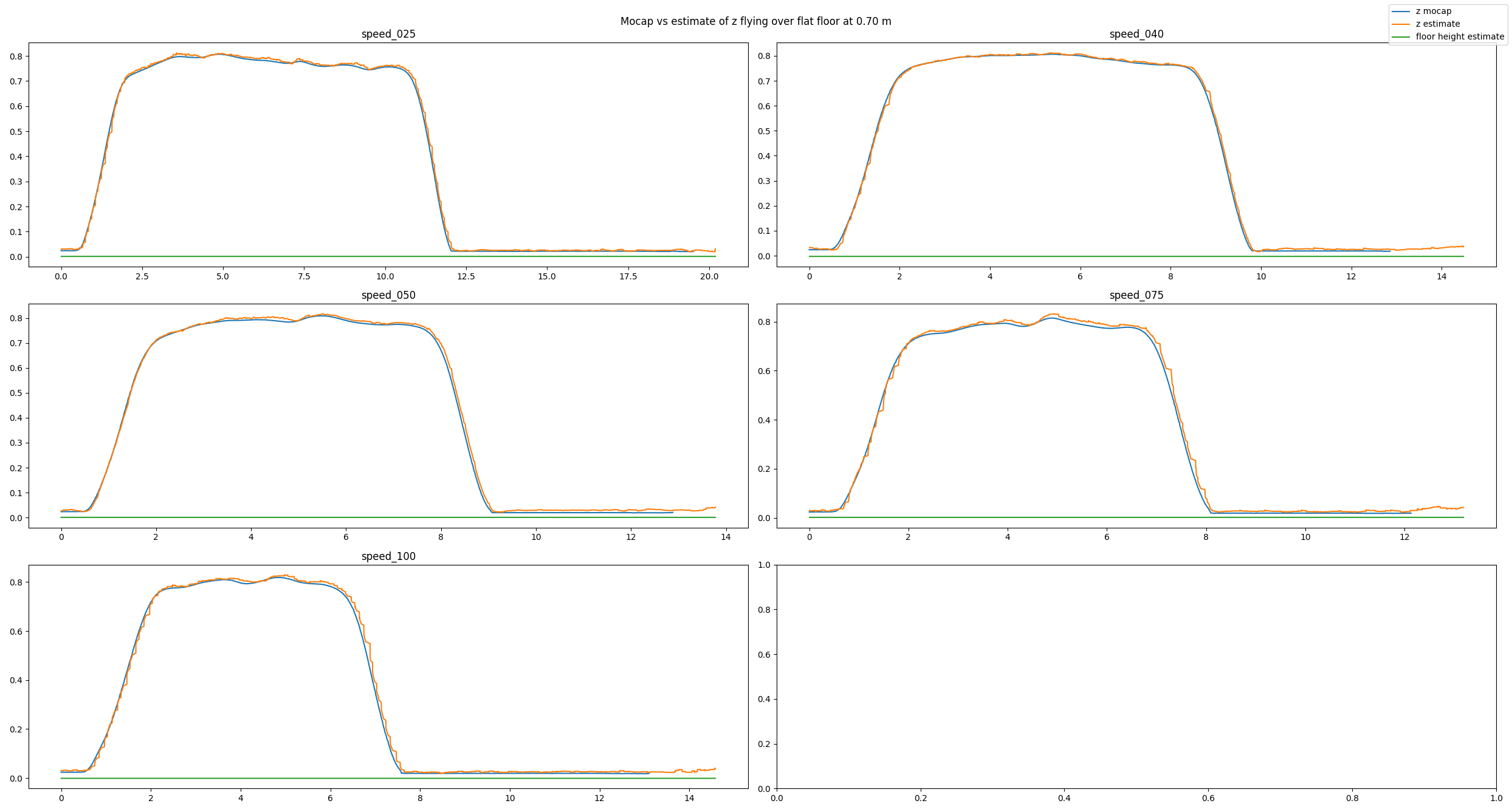
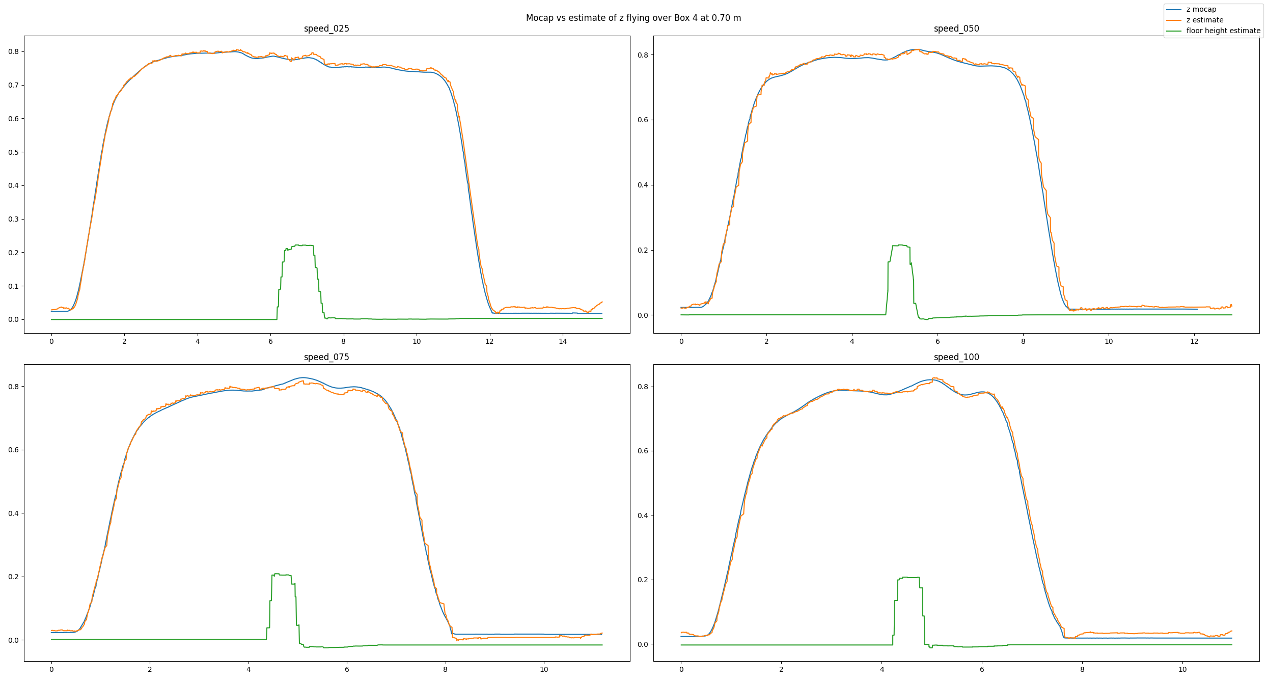
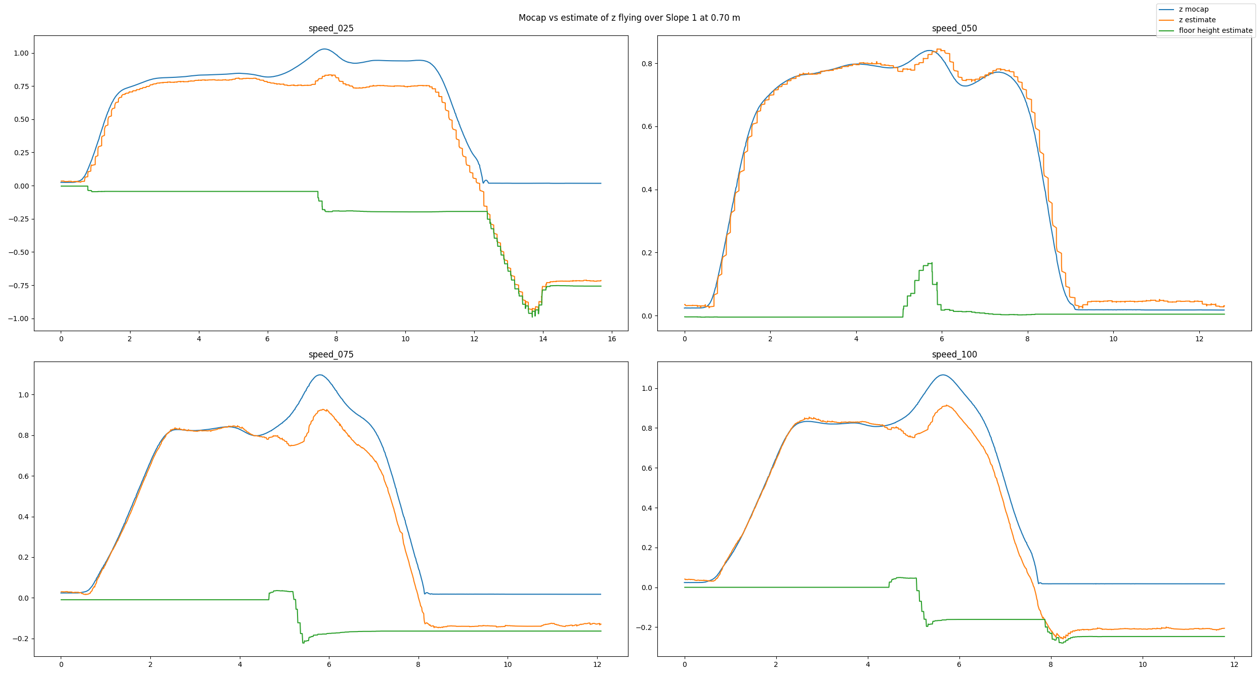
To analyze our approach we have used a Qualisys motion capture system. We have conducted many different tests: flying over different obstacles, flying at different velocities, flying at different altitudes, or even flying under different lighting conditions. Exemplarily, in this post we will have a look at a baseline example, a good estimate, and a bad estimate. In each picture you can see the altitude (in meters) over time (in seconds) for different flight speeds (in centimeters per second). You will see three lines: The motion capture ground truth (blue), the altitude estimated by our code (orange), and the new state keeping track of the floor height (green). For each plot, the Crazyflie takes off, flies in positive x direction, and lands.
In the baseline experiment, it flies over a flat floor. Clearly, the altitude estimates follow the ground truth values well, and the floor is correctly estimated to be flat.
Baseline experiment flying over a flat floor
In the next example, we have added a box with an approximate height of 0.225 m and made the Crazyflie fly over it. Despite the obstacle the altitude estimates follow the ground truth values well. Note how the floor estimates indicates the shape of the box.
Experiment flying over a box
Because the algorithm is based on an edge detection, we had a hunch that smoothly changing obstacles will pose a problem. Indeed, the estimates can be messy as we see in the next example. Here, the Crazyflie flies over an orthogonal triangle, with the short leg at 0.23 m pointing upwards and the long leg with 0.65 m pointing in flight direction (thus forming a slope). For different flight speeds different the estimates turn out quite differently.
Experiment flying over a slope
If you don’t like looking at plots, check out this video with some cool shots instead!
Conclusion
To summarize, we propose a solution for constant altitude flight with Crazyflies, using the Flow deck and the Multiranger deck. We have tested it successfully under various circumstances. Still, we see some potential for improvement, e.g. when dealing with slopes. In addition, the current implementation is quite a change to the original EKF, which poses a problem for integration.
Thus, a way forward can be an out-of-tree build to ease the use of the solution for the community. At SINTEF we certainly plan to deploy this code in all of our tests in 2022, which will hopefully allow us to gather more experience and thus find further ways to improve or tune the system.
We want to emphasize that this is not a perfect solution. That means a) you should use it with care and b) you are very much welcomed to contribute. E.g. feel free to chime in in the pull request, test the code in your environments, propose improvements, or implement an out-of-tree build! :) Maybe you can even come up with an alternative approach for constant altitude flights?
If you want to check out more of our work, visit our website. Also, keep reading this amazing blog from Bitcraze as we try to be back some day (if Bitcraze wants us hehe)!
From Star Wars to Black Mirror, sci-fi movies predict a future where thousands of drones will fill our sky. Curving sharply around trees or soaring over buildings, they fly just like a flock of starlings. To turn this vision into a reality, real drone swarms need to increase their autonomy and operate in a decentralized fashion. In a decentralized swarm, each robot makes its own decision based only on local information. Decentralization not only allows the swarm to be more robust to the failure of single individuals, but also removes the dependency from a single computing unit, thus making the swarm more scalable in terms of size.
We at LIS (EPFL) have shown that predictive controllers can improve the safety of aerial swarms by predicting and optimizing the agents’ future behavior in an iterative process. However, the centralized nature of this method allowed us to only control five drones and prevented us from scaling up to a large number of drones. For this reason, we have worked on a novel decentralized and scalable swarm controller that allows the safe and cohesive flight of aerial swarms in cluttered environments. In our latest article, published in IEEE Robotics and Automation Letters (RA-L), we describe how we designed the controller, show its scalability in size, and demonstrate its robustness to noise. We studied the swarms’ performance and compared how it changes in two different environments: a forest and funnel-like environment.
The Crazyflie 2.1 was the perfect platform for our experiments. They are lightweight, modular, and tough. This quadcopter can survive big hits when things don’t go as planned… and, if you work on swarms, things can go wrong!
The fleet of Crazyflies equipped with a single marker.
With our algorithm, sixteen robots were able to fly through an artificial forest that we set up in our indoor motion capture arena. In our previous work, we installed four markers on each quadcopter and used the rigid body tracking from Motive (the Optitrack software). The large volume of our experimental room required the usage of big markers for long-distance detection, which added considerable weight to the drone. Hence, in our new work, we use a single marker per drone. Tracking is supported by the ‘crazyswarm’ package and communication with the entire swarm only requires two radio links. However, despite our model being decentralized, in our implementation robots relay the information to an external brain, which does the computations for them. In the future, all the necessary code will be embedded onboard, removing the dependency on external infrastructure.
Our predictive swarm of Crazyflies flying among obstacles in our indoor experimental room.
Video about the article
This work is a step forward towards the fully autonomous deployment of drone swarms in our cities. By enabling safe navigation in cluttered environments, drone fleets will be able to integrate with conventional air traffic, search for missing people, inspect dangerous areas, transport injured people to hospitals quicker, and deliver important packages right to our doors.
This week we have a guest blog post from Bart Duisterhof and Prof. Guido de Croon from the MAVlab, Faculty of Aerospace Engineering from the Delft University of Technology. Enjoy!
Tiny drones are ideal candidates for fully autonomous jobs that are too dangerous or time-consuming for humans. A commonly shared dream would be to have swarms of such drones help in search-and-rescue scenarios, for instance to localize gas leaks without endangering human lives. Drones like the CrazyFlie are ideal for such tasks, since they are small enough to navigate in narrow spaces, safe, agile, and very inexpensive. However, their small footprint also makes the design of an autonomous swarm extremely challenging, both from a software and hardware perspective.
From a software perspective, it is really challenging to come up with an algorithm capable of autonomous and collaborative navigation within such tight resource constraints. State-of-the-art solutions like SLAM require too much memory and processing power. A promising line of work is to use bug algorithms [1], which can be implemented as computationally efficient finite state machines (FSMs), and can navigate around obstacles without requiring a map.
A downside of using FSMs is that the resulting behavior can be very sensitive to their hyperparameters, and therefore may not generalize outside of the tested environments. This is especially true for the problem of gas source localization (GSL), as wind conditions and obstacle configurations drastically change the problem. In this blog post, we show how we tackled the complex problem of swarm GSL in cluttered environments by using a simple bug algorithm with evolved parameters, and then tested it onboard a fully autonomous swarm of CrazyFlies. We will focus on the problems that were encountered along the way, and the design choices we made as a result. At the end of this post, we will also add a short discussion about the future of nano drones.
Why gas source localization?
Overall we are interested in finding novel ways to enable autonomy on constrained devices, like CrazyFlies. Two years ago, we showed that a swarm of CrazyFlie drones was able to explore unknown, cluttered environments and come back to the base station. Since then, we have been working on an even more complex task: using such a swarm for Gas Source Localization (GSL).
There has been a lot of research focussing on autonomous GSL in robotics, since it is an important but very hard problem. The difficulty of the task comes from the complexity of how odor can spread in an environment. In an empty room without wind, a gas will slowly diffuse from the source. This can allow a robot to find it by moving up gradient, just like small bacteria like E. Coli do. However, if the environment becomes larger with many obstacles and walls, and wind comes into play, the spreading of gas is much less regular. Large parts of the environment may have no gas or wind at all, while at the same time there may be pockets of gas away from the source. Moreover, chemical sensors for robots are much less capable than the smelling organs of animals. Available chemical sensors for robots are typically less sensitive, noisier, and much slower.
Due to these difficulties, most work in the GSL field has focused on a single robot that has to find a gas source in environments that are relatively small and without obstacles. Relatively recently, there have been studies in which groups of robots solve this task in a collaborative fashion, for example with Particle Swarm Optimization (PSO). This allows robots to find the source and escape local maxima when present. Until now this concept has been shown in simulation [2] and on large outdoor drones equipped with LiDAR and GPS [3], but never before on tiny drones in complex, GPS-denied, indoor environments.
Required Infrastructure
In our project, we introduce a new bug algorithm, Sniffy Bug, which uses PSO for gas source localization. In order to tune the FSM of Sniffy Bug, we used an artificial evolution. For time reasons, evolution typically takes place in simulation. However, early in the project, we realized that this would be a challenge, as no end-to-end gas modeling pipeline existed yet. It is important to have an easy-to-use pipeline that does not require any aerodynamics domain knowledge, such that as many researchers as possible can generate environments to test their algorithms. It would also make it easier to compare contributions and to better understand in which conditions certain algorithms work or don’t work. The GADEN ROS package [4] is a great open-source tool for modeling gas distribution when you have an environment and flow field, but for our objective, we needed a fully automated tool that could generate a great variety of random environments on-demand with just a few parameters. Below is an overview of our simulation pipeline: AutoGDM.
AutoGDM, a fully automated gas dispersion modeling (GDM) simulation pipeline.
First, we use a procedural environment generator proposed in [5] to generate random walls and obstacles inside of the environment. An important next step is to generate a 3D flowfield by means of computational fluid dynamics (CFD). A hard requirement for us was that AutoGDM needed to be free to use, so we chose to use the open-source CFD tool OpenFOAM. It’s used for cutting-edge aerodynamics research, and also the tool suggested by the authors of GADEN. Usually, using OpenFOAM isn’t trivial, as a large number of parameters need to be selected that require field expertise, resulting in a complicated process. Next, we integrate GADEN into our pipeline, to go from environment definition (CAD files) and a flow field to a gas concentration field. Other parts that needed to be automated were the random selection of boundary conditions, which has a large impact on the actual flow field, and source placement, which has an equally large impact on the concentration field.
After we built this pipeline, we started looking for a robot simulator to couple it to. Since we weren’t planning on using a camera, our main requirement was for the simulator to be efficient (preferably in 2D) so that evolutions would take relatively little time. We decided to use Swarmulator [6], a lightweight C++ robot simulator designed for swarming and we plugged in our gas data.
Algorithm Design
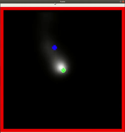
Roughly speaking, we considered two categories of algorithms for controlling the drones: 1) a neural network, and 2) an FSM that included PSO, with evolved parameters. Since we used a tiny neural network for light seeking with a CrazyFlie in our previous work, we first evolved neural networks in simulation. One of the first experiments is shown below.
A single agent in simulation seeking a light source using a tiny neural network.
While it worked pretty well in simple environments with few obstacles, it seemed challenging to make this work in real life with complex obstacles and multiple agents that need to collaborate. Given the time constraints of the project, we have opted for evolving the FSM. This also facilitated crossing the reality gap, as the simulated evolution could build on basic behaviors that we developed and validated on the real platform, including obstacle avoidance with four tiny laser rangers, while communicating with and avoiding other drones. An additional advantage of PSO with respect to the reality gap is that it only needs gas concentration and no gradient of the gas concentration or wind direction (which many algorithms in literature use). On a real robot at this scale, estimating the gas concentration gradient or the direction of a light breeze is hard if not impossible.
Hardware
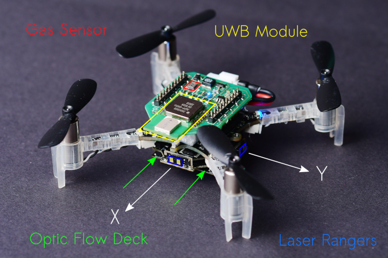
Our CrazyFlie needs to be able to avoid obstacles, execute velocity commands, sense gas, and estimate the other agent’s position in its own frame. For navigation, we added the flow deck and laser rangers, whereas for gas sensing we used a TGS8100 gas sensor that was used on a CrazyFlie before in previous work [7]. The sensor is lightweight and inexpensive, but accurately estimating gas concentrations can be difficult because of its size. It tends to drift and needs time to recover after a spike in concentration is observed. Another thing we noticed is that it is possible to break them, a crash can definitely destroy the sensor.
To estimate the relative position between agents, we use a Decawave Ultra-Wideband (UWB) module and communicate states, as proposed in [8]. We also use the UWB module to communicate gas information between agents and collaboratively seek the source. The complete configuration is visible below.
A 37.5 g nano quadcopter, capable of fully autonomous waypoint tracking, obstacle avoidance, relative localization, communication and gas sensing.
Evaluation in Simulation
After we optimized the parameters of our model using Swarmulator and AutoGDM, and of course trying many different versions of our algorithm, we ended up with the final Sniffy Bug algorithm. Below is a video that shows evolved Sniffy Bug evaluated in six different environments. The red dots are an agent’s personal target waypoint, whereas the yellow dot is the best-known position for the swarm.
Sniffy Bug evaluated in Swarmulator environments.
Simulation showed that Sniffy Bug is effective at locating the gas source in randomly generated environments. The drones successfully collaborate by means of PSO.
Real Flight Testing
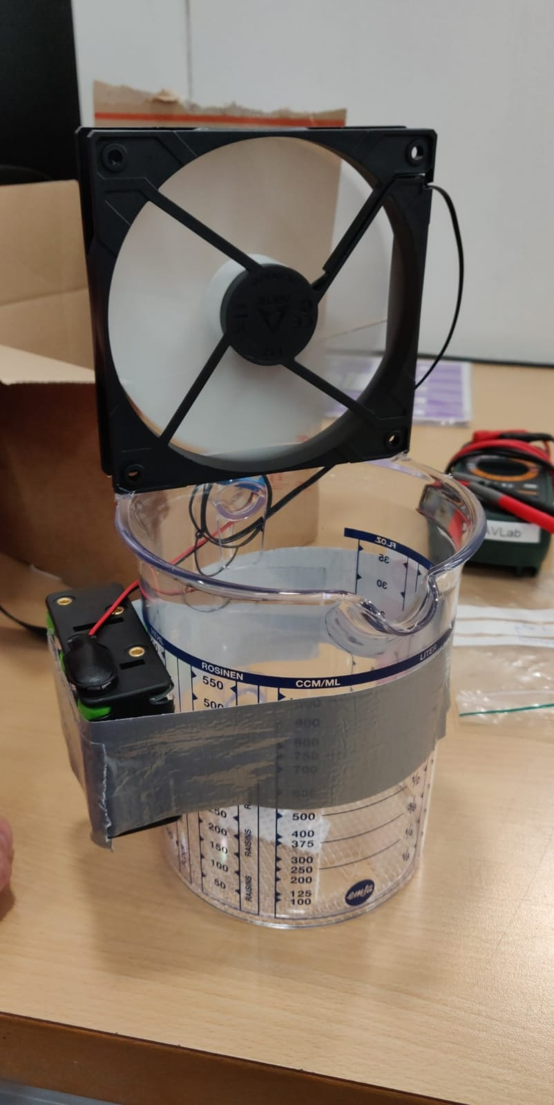
After observing Sniffy Bug in simulation we were optimistic, but unsure about performance in real life. First, inspired by previous works, we disperse alcohol through the air by placing liquid alcohol into a can which is then dispersed using a computer fan.
Dispersion of liquid alcohol in flight tests.
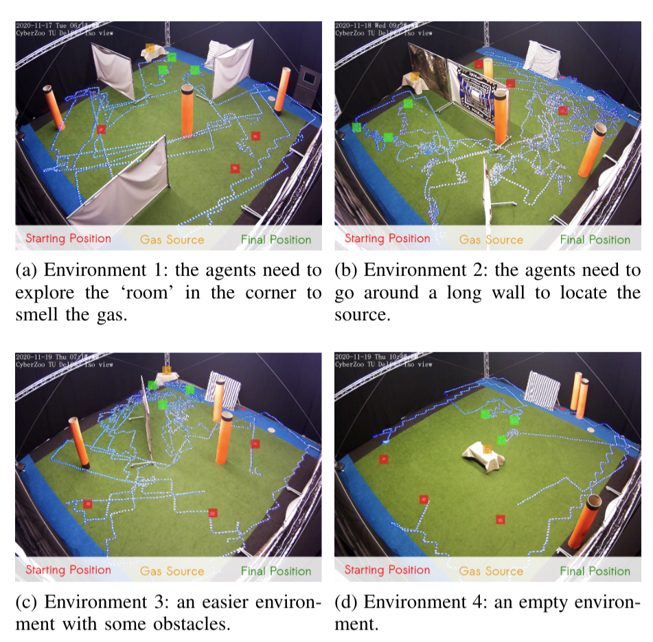
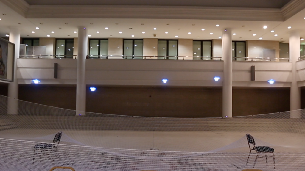
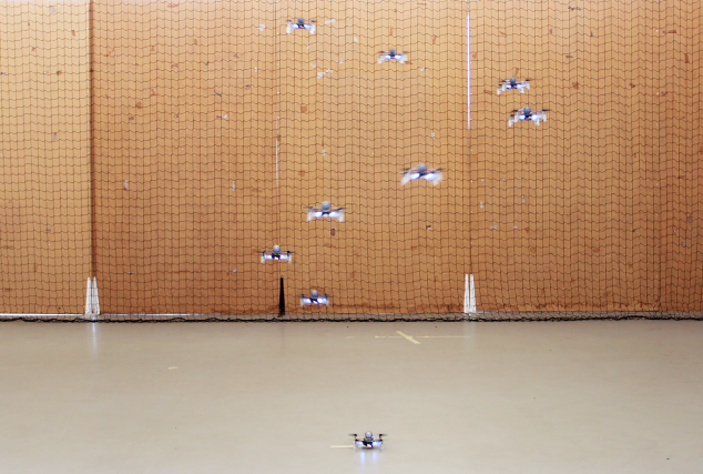
We test Sniffy Bug in our flight arena of size 10 x 10 meters with large obstacles that are shaped like walls and orange poles. The image below shows four flight tests of Sniffy Bug in cluttered environments, flying fully autonomously, i.e., without the help from any external infrastructure.
Time-lapse images of real-world experiments in our flight arena. Sniffy was evaluated on four distinct environments, 10 x 10 meters in size, seeking a real isopropyl alcohol source. The trajectories of the nano quadcopters are clearly visible due to their blue lights.
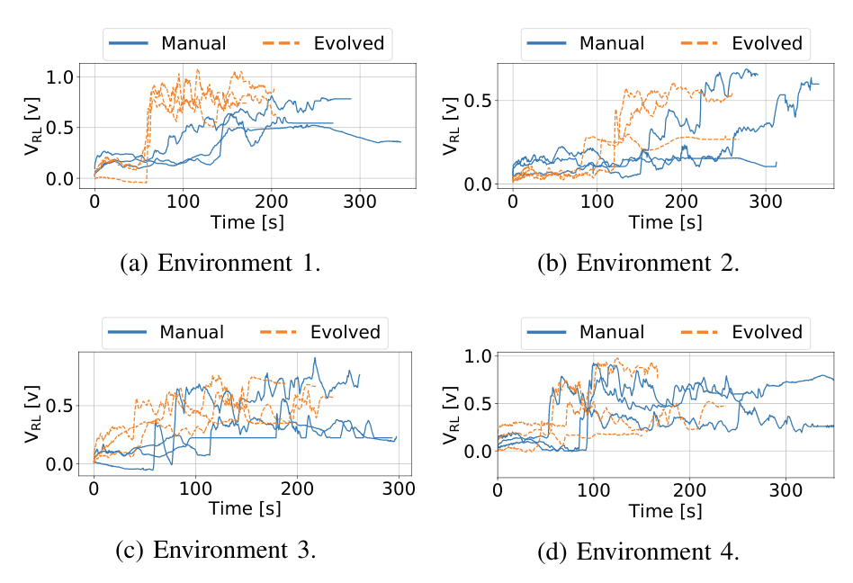
In the total of 24 runs we executed, we compared Sniffy Bug with manually selected and evolved parameters. The figure below shows that the evolved parameters are more efficient in locating the source as compared to the manual parameters.
Maximum recorded gas reading by the swarm, for each time step for each run.
This does not only show that our system can successfully locate a gas source in challenging environments, but it also demonstrates the usefulness of the simulation pipeline. The parameters that were learned in simulation yield a high-performance model, validating the environment generation, randomization, and gas modeling parts of our pipeline.
Conclusion and Discussion
With this work, we believe we have made an important step towards swarms of gas-seeking drones. The proposed solution is shown to work in real flight tests with obstacles, and without any external systems to help in localization or communication. We believe this methodology can be extended to larger environments or even to 3 dimensions, since PSO is a robust, multi-dimensional heuristic search method. Moreover, we hope that AutoGDM will help the community to better compare gas seeking algorithms, and to more easily learn parameters or models in simulation, and deploy them in the real world.
To improve Sniffy Bug’s performance, adding more laser rangers will definitely help. When working with only four laser rangers you realize how little information it actually provides. If one of the rangers senses a low value it is unclear if a slim pole or a massive wall is detected, adding inefficiency to the algorithm. Adding more laser rangers or using other sensor modalities like vision will help to avoid also more complex obstacles than walls and poles in a reliable manner.
Another interesting discussion can be held on the hardware required for real deployment. When working with 40 grams of maximum take-off weight, the sensors and actuators that can be selected are limited. For example, the low-power and lightweight flow deck works great but fails in low-light scenarios or with smoke. Future work exploring novel sensors for highly constrained nano robots could really help increase the Technological Readiness Level (TRL) of these systems.
Finally, this has been a really fun project to work on for us and we can’t wait to hear your thoughts on Sniffy Bug!
This week we have a guest blog post from Dr Feng Shan at School of Computer Science and Engineering Southeast University, China. Enjoy!
It is possible to utilize tens and thousands of Crazyflies to form a swarm to complete complicated cooperative tasks, such as searching and mapping. These Crazyflies are in short distance to each other and may move dynamically, so we study the dynamic and dense swarms. The ultra-wideband (UWB) technology is proposed to serve as the fundamental technique for both networking and localization, because UWB is so time sensitive that an accurate distance can be calculated using the transmission and receive timestamps of data packets. We have therefore designed a UWB Swarm Ranging Protocol with key features: simple yet efficient, adaptive and robust, scalable and supportive. It is implemented on Crazyflie 2.1 with onboard UWB wireless transceiver chips DW1000.
Fig.1. Nine Crazyflies are in a compact space ranging the distance with each other.
The Basic Idea
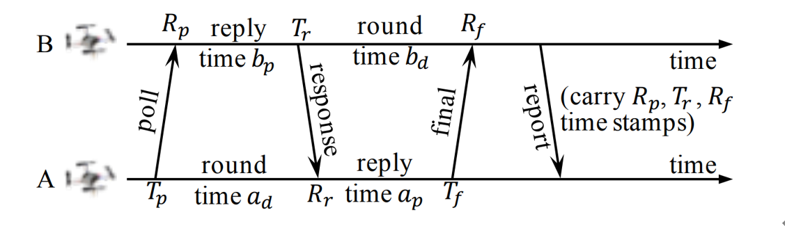
The basic idea of the swarm ranging protocol was inspired by Double Sided-Two Way Ranging (DS-TWR), as shown below.
Fig.2. The exsiting Double Sided-Two Way Ranging (DS-TWR) protocol.
There are four types of message in DS-TWR, i.e., poll, response, final and report message, exchanging between the two sides, A and B. We define their transmission and receive timestamps are Tp, Rp, Tr, Rr, Tf, and Rf, respectively. We define the reply and round time duration for the two sides as follows.
Let tp be the time of flight (ToF), namely radio signal propagation time. ToF can be calculated as Eq. (2).
Then, the distance can be estimated by the ToF.
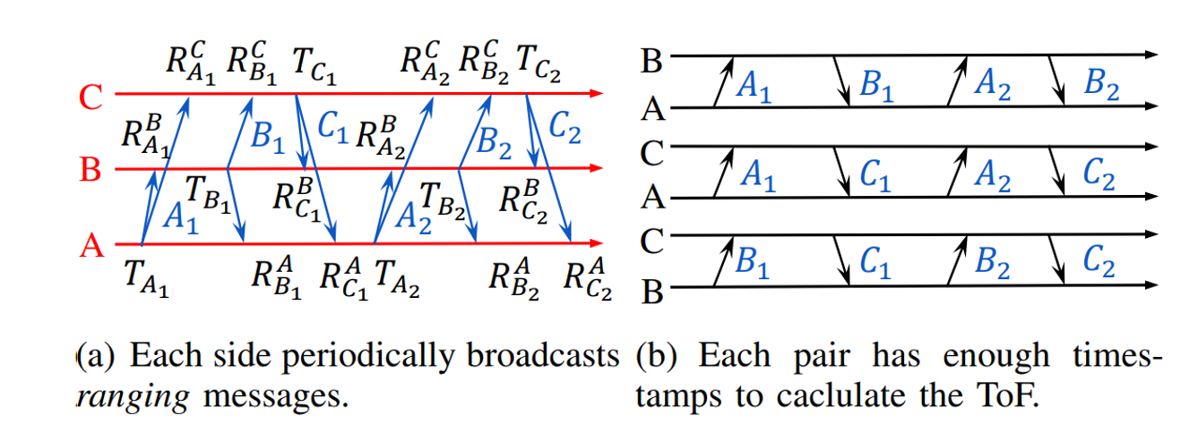
In our proposed Swarm Ranging Protocol, instead of four types of messages, we use only one type of message, which we call the ranging message.
Fig.3. The basic idea of the proposed Swarm Ranging Protocol.
Three sides A, B and C take turns to transmit six messages, namely A1, B1, C1, A2, B2, and C2. Each message can be received by the other two sides because of the broadcast nature of wireless communication. Then every message generates three timestamps, i.e., one transmission and two receive timestamps, as shown in Fig.3(a). We can see that each pair has two rounds of message exchange as shown in Fig.3(b). Hence, there are sufficient timestamps to calculate the ToF for each pair, that means all three pairs can be ranged with each side transmitting only two messages. This observation inspires us to design our ranging protocol.
Protocol Design
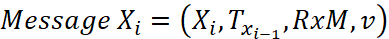
The formal definition of the i-th ranging message that broadcasted by Crazyflie X is as follows.
Xi is the message identification, e.g., sender and sequence number; Txi-1 is the transmission timestamp of Xi-1, i.e., the last sent message; RxM is the set of receive timestamps and their message identification, e.g., RxM = {(A2, RA2), (B2, RB2)}; v is the velocity of X when it generates message Xi.
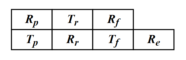
As mentioned above, six timestamps (Tp, Rp, Tr, Rr, Tf, Rf,) are needed to calculate the ToF. Therefore, for each neighbor, an additional data structure is designed to store these timestamps which we named it the ranging table, as shown in Fig.4. Each device maintains one ranging table for each known neighbor to store the timestamps required for ranging.
Fig.4. The ranging table, one for each neighbor.
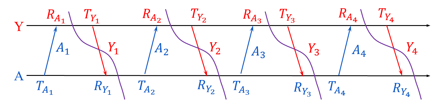
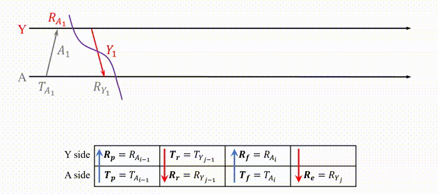
Let’s focus on a simple scenario where there are a number of Crazyflies, A, B, C, etc, in a short distance. Each one of them transmit a message that can be heard by all others, and they broadcast ranging messages at the same pace. As a result, between any two consecutive message transmission, a Crazyflie can hear messages from all others. The message exchange between A and Y is as follows.
Fig.5. Message exchange between A and Y.
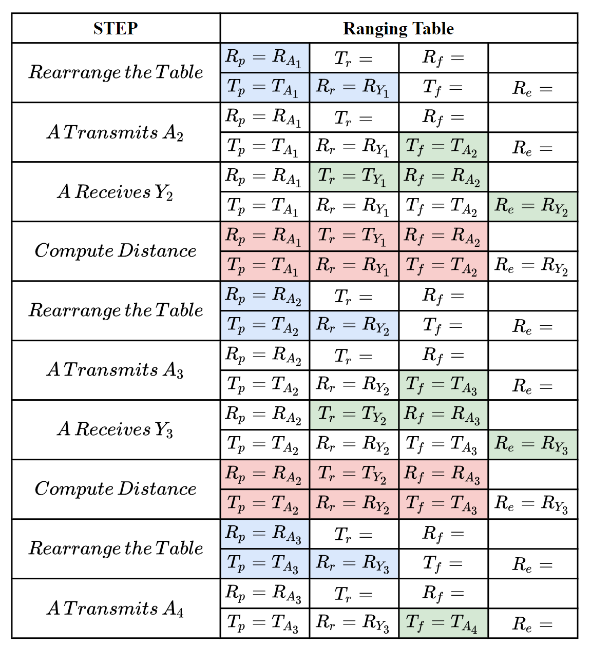
The following steps show how the ranging messages are generated and the ranging tables are updated to correctly compute the distance between A and Y.
Fig.6. How the ranging message and ranging table works to compute distance.
The message exchange between A and Y could be also A and B, A and C, etc, because they are equal, that’s means A could perform the ranging process above with all of it’s neighbors at the same time.
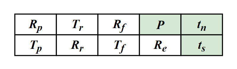
To handle dense and dynamic swarm, we improved the data structure of ranging table.
Fig.7. The improved ranging table for dense and dynamic swarm.
There are three new notations P, tn, ts, denoting the newest ranging period, the next (expected) delivery time and the expiration time, respectively.
For any Crazyflie, we allow it to have different ranging period for different neighbors, instead of setting a constant period for all neighbors. So, not all neighbors’ timestamps are required to be carried in every ranging message, e.g., the receive timestamp to a far apart and motionless neighbor is required less often. tn is used to measure the priority of neighbors. Also, when a neighbor is not heard for a certain duration, we set it as expired and will remove its ranging table.
If you are interested in our protocol, you can find much more details in our paper, that has just been published on IEEE International Conference on Computer Communications (INFOCOM) 2021. Please refer the links at the bottom of this article for our paper.
Implementation
We have implemented our swarm ranging protocol for Crazyflie and it is now open-source. Note that we have also implemented the Optimized Link State Routing (OLSR) protocol, and the ranging messages are one of the OLSR messages type. So the “Timestamp Message” in the source file is the ranging message introduced in this article.
The procedure that handles the ranging messages is triggered by the hardware interruption of DW1000. During such procedure, timestamps in ranging tables are updated accordingly. Once a neighbor’s ranging table is complete, the distance is calculated and then the ranging table is rearranged.
All our codes are stored in the folder crazyflie-firmware/src/deck/drivers/src/swarming.
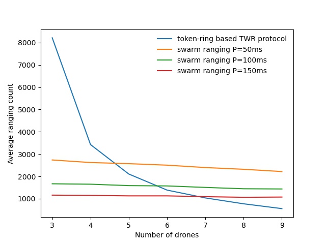
The following figure is a ranging performance comparison between our ranging protocol and token-ring based TWR protocol. It’s clear that our protocol handles the large number of drones smoothly.
Fig.8. performance comparison.
We also conduct a collision avoidance experiment to test the real time ranging accuracy. In this experiment, 8 Crazyflie drones hover at the height 70cm in a compact area less than 3m by 3m. While a ninth Crazyflie drone is manually controlled to fly into this area. Thanks to the swarm ranging protocol, a drone detects the coming drone by ranging distance, and lower its height to avoid collision once the distance is small than a threshold, 30cm.
cd crazyflie-firmware/src/deck/drivers/src/swarming
Then build the firmware.
make clean
make
Flash the cf2.bin.
cfloader flash path/to/cf2.bin stm32-fw
Open the client, connect to one of the drones and add log variables. (We use radio channel as the address of the drone) Our swarm ranging protocol allows the drones to ranging with multiple targets at the same time. The following shows that our swarm ranging protocol works very efficiently.
Summary
We designed a ranging protocol specially for dense and dynamic swarms. Only a single type of message is used in our protocol which is broadcasted periodically. Timestamps are carried by this message so that the distance can be calculated. Also, we implemented our proposed ranging protocol on Crazyflie drones. Experiment shows that our protocol works very efficiently.
This week we have a guest blog post from Wenda Zhao, Ph.D. candidate at the Dynamic System Lab (with Prof. Angela Schoellig), University of Toronto Institute for Aerospace Studies (UTIAS). Enjoy!
Accurate indoor localization is a crucial enabling capability for indoor robotics. Small and computationally-constrained indoor mobile robots have led researchers to pursue localization methods leveraging low-power and lightweight sensors. Ultra-wideband (UWB) technology, in particular, has been shown to provide sub-meter accurate, high-frequency, obstacle-penetrating ranging measurements that are robust to radio-frequency interference, using tiny integrated circuits. UWB chips have already been included in the latest generations of smartphones (iPhone 12, Samsung Galaxy S21, etc.) with the expectation that they will support faster data transfer and accurate indoor positioning, even in cluttered environments.
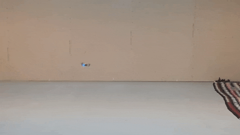
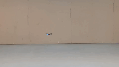
A Crazyflie with an IMU and UWB tag flies through a cardboard tunnel. A vision-based motion capture system would not be able to achieve this due to the occlusion.
In our lab, we show that a Crazyflie nano-quadcopter can stably fly through a cardboard tunnel with only an IMU and UWB tag, from Bitcraze’s Loco Positioning System (LPS), for state estimation. However, it is challenging to achieve a reliable localization performance as we show above. Many factors can reduce the accuracy and reliability of UWB localization, for either two-way ranging (TWR) or time-difference-of-arrival (TDOA) measurements. Non-line-of-sight (NLOS) and multi-path radio propagation can lead to erroneous, spurious measurements (so-called outliers). Even line-of-sight (LOS) UWB measurements exhibit error patterns (i.e., bias), which are typically caused by the UWB antenna’s radiation characteristics. In our recent work, we present an M-estimation-based robust Kalman filter to reduce the influence of outliers and achieve robust UWB localization. We contributed an implementation of the robust Kalman filter for both TWR and TDOA (PR #707 and #745) to Bitcraze’s crazyflie-firmware open-source project.
Methodology
The conventional Kalman filter, a primary sensor fusion mechanism, is sensitive to measurement outliers due to its minimum mean-square-error (MMSE) criterion. To achieve robust estimation, it is critical to properly handle measurement outliers. We implement a robust M-estimation method to address this problem. Instead of using a least-squares, maximum-likelihood cost function, we use a robust cost function to downweigh the influence of outlier measurements [1]. Compared to Random Sample Consensus (RANSAC) approaches, our method can handle sparse UWB measurements, which are often a challenge for RANSAC.
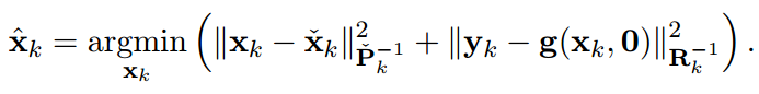
From the Bayesian maximum-a-posteriori perspective, the Kalman filter state estimation framework can be derived by solving the following minimization problem:
Therein, xk and yk are the system state and measurements at timestep k. Pk and Rk denote the prior covariance and measurement covariance, respectively. The prior and posteriori estimates are denoted as xk check and xk hat and the measurement function without noise is indicated as g(xk,0). Through Cholesky factorization of Pk and Rk, the original optimization problem is equivalent to
where ex,k,i and ey,k,j are the elements of ex,k and ey,k. To reduce the influence of outliers, we incorporate a robust cost function into the Kalman filter framework as follows:
where rho() could be any robust function (G-M, SC-DCS, Huber, Cauchy, etc.[2]).
By introducing a weight function for the process and measurement uncertainties—with e as input—we can translate the optimization problem into an Iteratively Reweighted Least Squares (IRLS) problem. Then, the optimal posteriori estimate can be computed through iteratively solving the least-squares problem using the robust weights computed from the previous solution. In our implementation, we use the G-M robust cost function and the maximum iteration is set to be two for computational reasons. For further details about the robust Kalman filter, readers are referred to our ICRA/RA-L paper and the onboard firmware (mm_tdoa_robust.c and mm_distance_robust.c).
Performance
We demonstrate the effectiveness of the robust Kalman filter on-board a Crazyflie 2.1. The Crazyflie is equipped with an IMU and an LPS UWB tag (in TDOA2 mode). With the conventional onboard extended Kalman filter, the drone is affected by measurement outliers and jumps around significantly while trying to hover. In contrast, with the robust Kalman filter, the drone shows a more reliable localization performance.
Conventional extended Kalman filter
M-estimation-based robust Kalman filter
Quadcopter is commanded to hover. UWB TDOA-based localization performance of standard method on-board a Crazyflie 2.1 quadcopter (left) and the proposed robust Kalman filter (right).
The robust Kalman filter implementations for UWB TWR and TDOA localization have been included in the crazyflie-firmware master branch as of March 2021 (2021.03 release). This functionality can be turned on by setting a parameter (robustTwr or robustTdoa) in estimator_kalman.c. We encourage LPS users to check out this new functionality.
As we mentioned above, off-the-shelf, low-cost UWB modules also exhibit distinctive and reproducible bias patterns. In our recent work, we devised experiments using the LPS UWB modules and showed that the systematic biases have a strong relationship with the pose of the tag and the anchors as they result from the UWB radio doughnut-shaped antenna pattern. A pre-trained neural network is used to approximate the systematic biases. By combining bias compensation with the robust Kalman filter, we obtain a lightweight, learning-enhanced localization framework that achieves accurate and reliable UWB indoor positioning. We show that our approach runs in real-time and in closed-loop on-board a Crazyflie nano-quadcopter yielding enhanced localization performance for autonomous trajectory tracking. The dataset for the systematic biases in UWB TDOA measurements is available on our Open-source Code & Dataset webpage. We are also currently working on a more comprehensive dataset with IMU, UWB, and optical flow measurements and again based on the Crazyflie platform. So stay tuned!
Reference
[1] L. Chang, K. Li, and B. Hu, “Huber’s M-estimation-based process uncertainty robust filter for integrated INS/GPS,” IEEE Sensors Journal, 2015, vol. 15, no. 6, pp. 3367–3374.
[2] K. MacTavish and T. D. Barfoot, “At all costs: A comparison of robust cost functions for camera correspondence outliers,” in IEEE Conference on Computer and Robot Vision (CRV). 2015, pp. 62–69.
Feel free to contact us if you have any questions or suggestions: wenda.zhao@robotics.utias.utoronto.ca.
Please cite this as:
<code>@ARTICLE{Zhao2021Learningbased,
author={W. {Zhao} and J. {Panerati} and A. P. {Schoellig}},
title={Learning-based Bias Correction for Time Difference of Arrival Ultra-wideband Localization of Resource-constrained Mobile Robots},
journal={IEEE Robotics and Automation Letters},
volume={6},
number={2},
pages={3639-3646},
year={2021},
publisher={IEEE}
doi={10.1109/LRA.2021.3064199}}
</code>
Since the middle of January, Bitcraze has had two additional guests: us! We, Josefine & Max, are currently doing our master thesis at Bitcraze during our final semester at LTH.
Unfortunately, the pandemic means remote working which could have caused some difficulties with hardware and equipment accessibility. Fortunately, for us, our goal with the thesis is to emulate the Crazyflie 2.1 hardware in the open source software Renode. We can therefore do the work at home.
Since this is the first time either of us have tried to emulate hardware it is exciting to see if it will even be possible, especially as we do not know what limitations Renode might have. Thus far, four weeks in, there have been some hiccups and crashes but also progress and success. One example was when we got the USART up and running and it became possible to start printing debug messages and another was when the LED lights were connected and it was possible to see when they were turned on and off.
Example of output from partially implemented hardware.
If all goes well, the emulated hardware could be used as a part of the CI pipeline to automatically hunt for bugs. Academically, it would be used to further study testing methods of control firmware.
Getting a glimpse into the workings at Bitcraze and the lovely people working here has been most interesting and we are looking forward to the time ahead. Until next time, hopefully with a working emulation, Josefine & Max.
This week we have a guest blog post from CollMot about their work to integrate the Crazyflie with Skybrush. We are happy that they have used the app API that we wrote about a couple of weeks ago, to implement the required firmware extensions!
Bitcraze and CollMot have joined forcesto release an indoor drone show management solution using CollMot’s new Skybrush softwareand Crazyflie firmware and hardware.
CollMot is a drone show provider company from Hungary, founded by a team of researchers with a decade-long expertise in drone swarm science. CollMot offers outdoor drone shows since 2015. Our new product, Skybrush allows users to handle their own fleet-level drone missions and specifically drone shows as smoothly as possible. In joint development with the Bitcraze team we are very excited to extend Skybrush to support indoor drone shows and other fleet missions using the Crazyflie system.
The basic swarm-induced mindset with which we are targeting the integration process is scalability. This includes scalability of communication, error handling, reliability and logistics. Each of these aspects are detailed below through some examples of the challenges we needed to solve together. We hope that besides having an application-specific extension of Crazyflie for entertainment purposes, the base system has also gained many new features during this great cooperative process. But lets dig into the tech details a bit more…
UWB in large spaces with many drones
We have set up a relatively large area (10x20x6 m) with the Loco Positioning System using 8 anchors in a more or less cubic arrangement. Using TWR mode for swarms was out of question as it needs each tag (drone) to communicate with the anchors individually, which is not scalable with fleet size. Initial tests with the UWB system in TDoA2 mode were not very satisfying in terms of accuracy and reliability but as we went deeper into the details we could find out the two main reasons of inaccuracies:
Two of the anchors have been positioned on the vertical flat faces of some stairs with solid material connection between them that caused many reflections so the relative distance measurements between these two anchors was bi-stable. When we realized that, we raised them a bit and attached them to columns that had an air gap in between, which solved the reflection issue.
The outlier filter of the TDoA2 mode was not optimal, a single bad packet generated consecutive outliers that opened up the filter too fast. This issue have been solved since then in the Crazyflie firmware after our long-lasting painful investigation with changing a single number from 2 to 3. This is how a reward system works in software development :)
After all, UWB was doing its job quite nicely in both TDoA2 and TDoA3 modes with an accuracy in the 10-20 cm level stably in such a large area, so we could move on to tune the controller of the Crazyflie 2.1 a bit.
Crazyflies with Loco and LED decks
As we prepared the Crazyflie drones for shows, we had the Loco deck attached on top and the LED deck attached to the bottom of the drones, with an extra light bulb to spread light smoothly. This setup resulted in a total weight of 37g. The basic challenge with the controller was that this weight turned out to be too much for the Crazyflie 2.1 system. Hover was at around 60-70% throttle in average, furthermore, there was a substantial difference in the throttle levels needed for individual motors (some in the 70-80% range). The tiny drones did a great job in horizontal motion but as soon as they needed to go up or down with vertical speed above around 0.5 m/s, one of their ESCs saturated and thus the system became unstable and crashed. Interestingly enough, the crash always started with a wobble exactly along the X axis, leading us to think that there was an issue with the positioning system instead of the ESCs. There are two possible solutions for this major problem:
use less payload, i.e. lighter drones
use stronger motors
Partially as a consequence of these experiments the Bitcraze team is now experimenting with new stronger models that will be optimized for show use cases as well. We can’t wait to test them!
Optimal controller for high speeds and accurate trajectory following
In general we are not yet very satisfied with any of the implemented controllers using the UWB system for a show use-case. This use-case is special as trajectory following needs to be as accurate as possible both in space and time to avoid collisions and to result in nice synchronized formations, while maximal speed both horizontally and vertically have to be as high as possible to increase the wow-effect of the audience.
The PID controller has no cutoffs in its outputs and with the sometimes present large positioning errors in the UWB system controller outputs get way too large. If gains are reduced, motion will be sluggish and path is not followed accurately in time.
The Mellinger and INDI controllers work well only with positioning systems of much better accuracy.
We stuck with the PID controller so far and added velocity feed forward terms, cutoffs in the output and some nonlinearity in case of large errors and it helped a bit, but the solution is not fully satisfying. Hopefully, these modifications might be included in the main firmware soon. However, having a perfect controller with UWB is still an open question, any suggestions are welcome!
Show specific improvements in the firmware
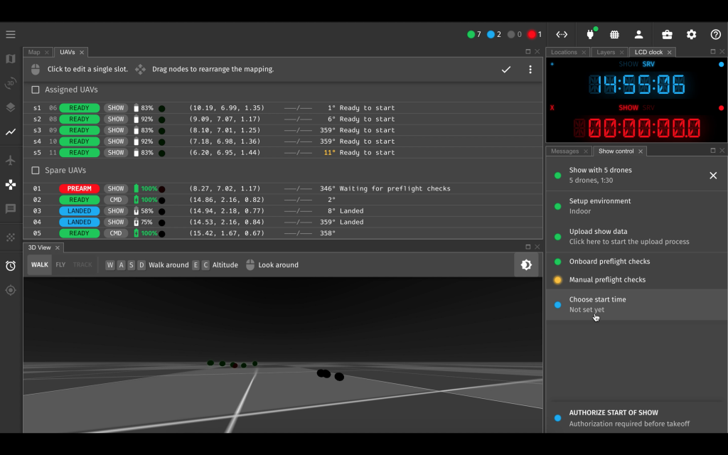
We implemented code that uploads the show content to the drones smoothly, performs automatic preflight checking and displays status with the LED deck to have visual feedback on many drones simultaneously, starts the show on time in synchrony with all swarm members and handles the light program and show trajectory execution of the show.
These modifications are now in our own fork of the Crazyflie firmware and will be rewritten soon into a show app thanks to this new promising possibility in the code framework. As soon as Skybrush and Crazyflie systems will be stable enough to be released together, we will publish the related app code that helps automating show logistics for every user.
Summary
To sum it up, we are very enthusiastic about the Crazyflie system and the great team behind the scenes with very friendly, open and cooperative support. The current stage of Crazyflie + Skybrush integration is as follows:
New hardware iterations based on the Bolt system that support longer and more dynamic flights are coming;
a very stable, UWB-compatible controller is still an open question but current possibilities are satisfying for initial tests with light flight dynamics;
a new Crazyflie app for the drone show case is basically ready to be launched together with the release of Skybrush in the near future.
If you are interested in Skybrush or have any questions related to this integration process, drop us an email or comment below.
This week we have a guest blog post from Bárbara Barros Carlos, PhD candidate at DIAG Robotics Lab. Enjoy!
Quadrotors are characterized by their underactuation, nonlinearities, bounded inputs, and, in some cases, communication time-delays. The development of their maneuvering capability poses some challenges that cover dynamics modeling, state estimation, trajectory generation, and control. The latter, in particular, must be able to exploit the system’s nonlinear dynamics to generate complex motions. However, the presence of communication time-delay is known to highly degrade control performance.
A composite image showing our real-time NMPC with time-delay compensation being used on the Crazyflie during the tracking of a helical trajectory.
In our recent work, we present an efficient position control architecture based on real-time nonlinear model predictive control (NMPC) with time-delay compensation for quadrotors. Given the current measurement, the state is predicted over the delay time interval using an integrator and then passed to the NMPC, which takes into account the input bounds. We demonstrate the capabilities of our architecture using the Crazyflie 2.1 nano-quadrotor.
Time-Delay Compensation
In our aerial system, because of the radio communication latency, we have delays both in receiving measurements and sending control inputs. Likewise, since we intend to use NMPC, the potentially high computational burden associated with its solution becomes an element that must also be taken into account to minimize the error in the state prediction.
Crazyflie NMPC response without considering the time-delay compensation.
To tackle this issue, we use a state predictor based on the round-trip time (RTT) associated with the sum of network latencies as a delay compensator. The prediction is computed by performing forward iterations of the system dynamic model, starting from the current measured state and over the RTT, through an explicit Runge Kutta 4th order (ERK4) integrator. Due to the independent nature of this operation, perfect delay compensation can be achieved by adjusting the integration step to be equal to the RTT. Thus, it is assumed that there is a fixed RTT, defined by τr, to be compensated.
Nonlinear Model Predictive Control
The NMPC controller is defined as the following constrained nonlinear program (NLP):
Therein, p denotes the inertial position, q the attitude in unit quaternions, vb the linear velocity expressed in the body frame, ω the angular rate, and Ωi the rotational speed of the ith propeller. The NLP is tailored to the Crazyflie 2.1 and is implemented using the high-performance software package acados, which solves optimal control problems and implements a real-time iteration (RTI) variant of a sequential quadratic programming (SQP) scheme with Gauss-Newton Hessian approximation. The quadratic subproblems (QP) arising in the SQP scheme are solved with HPIPM, an interior-point method solver, built on top of the linear algebra library BLASFEO, finely tuned for multiple CPU architectures. We use a recently proposed Hessian condensing algorithm particularly suitable for partial condensing to further speed-up solution times.
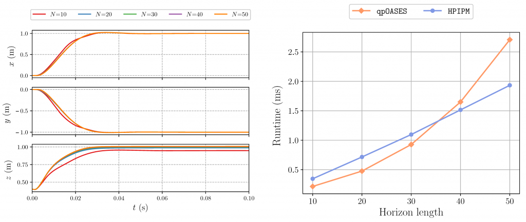
When designing an NMPC, choosing the horizon length has profound implications for computational burden and tracking performance. For the former, the longer the horizon, the higher the computational burden. As for the latter, in principle, a long prediction horizon tends to improve the overall performance of the controller. In order to select this parameter and achieve a trade-off between performance and computational burden, we implemented the NLP in acados considering: five horizon lengths (N = {10,20,30,40,50}), input bounds on the rotational speed of the propellers (lower bound = 0, upper bound = 22 krpm), discretizing the dynamics using an ERK4 integration scheme. Likewise, we compare the condensing approach with the state-of-the-art solver qpOASES against the partial condensing approach with HPIPM, concerning the set of horizons regarded.
Left: closed-loop trajectories comparing different horizon lengths. Right: average runtimes per SQP-iteration for different horizon lengths considering two distinct QP solvers.
As qpOASES is a solver based on active-set method, it requires condensing to be computationally efficient. In line with the observations found in the literature that condensing is effective for short to medium horizon lengths, we note that qpOASES is competitive for horizons up to approximately N = 30 when compared to HPIPM. The break-even point moves higher on the scale for longer horizons, mainly due to efficient software implementations that cover: (a) Hessian condensing procedure tailored for partial condensing, (b) structure-exploiting QP solver based on novel Riccati recursion, (c) hardware-tailored linear algebra library. Therefore, we chose horizon N = 50 as it offers a reasonable trade-off between deviation from the reference trajectory and computational burden.
Onboard Controller Considerations
How the onboard controllers (PIDs) use the setpoints of the offboard controller (NMPC) in our architecture is not entirely conventional and, thereby, deserves some considerations. First, the reference signals that the PID loops track do not fully correspond to the control inputs considered in the NMPC formulation. Instead, part of the state solution is used in conjunction with the control inputs to reconstruct the actual input commands passed as a setpoint to the Crazyflie. Second, a part of the reconstructed input commands is sent as a setpoint to the outer loop (attitude controller), and the other part is sent to the inner loop (rate controller). Furthermore, as the NMPC model does not include the PID loops, it does not truly represent the real system, even in the case of perfect knowledge of the physical parameters. As a consequence, the optimal feedback policy is distorted in the real system by the PIDs.
Closed-loop Position Control Performance
Our control architecture hinges upon a ROS Kinetic framework and runs at 66.67 Hz. The Crazy RealTime Protocol (CRTP) is used in combination with our crazyflie_nmpc stack to stream in runtime custom packages containing the required data to reconstruct the part of the measurement vector that depends on the IMU data. Likewise, the cortex_ros bridge streams the 3D global position of the Crazyflie, which is then passed through a second-order, discrete-time Butterworth filter to estimate the linear velocities.
To validate the effectiveness of our control architecture, we ran two experiments. For each experiment, we generate a reference trajectory on a base computer and pass it to our NMPC ROS node every τs = 15 ms. When generating the trajectories, we explicitly address the feasibility issue in the design process, creating two references: one feasible and one infeasible. In addressing this issue, we prove through experiments that the performance of the proposed NMPC is not degraded even when the nano-quadrotor attempts to track an infeasible trajectory, which could, in principle, make it deviate significantly or even crash.
Overall, we observe that the most challenging setpoints to be tracked are the positions in which, given a change in the motion, the Crazyflie has to pitch/roll in the opposite direction quickly. These are the setpoints where the distortion has the greatest influence on the system, causing small overshoots in position. The average solution time of the tailored RTI scheme using acados was obtained on an Intel Core i5-8250U @ 3.4 GHz running Ubuntu and is about 7.4 ms. This result shows the efficiency of the proposed scheme.
Outlook
In this work, we presented the design and implementation of a novel position controller based on nonlinear model predictive control for quadrotors. The control architecture incorporates a predictor as a delay compensator for granting a delay-free model in the NMPC formulation, which in turn enforces bounds on the actuators. To validate our architecture, we implemented it on the Crazyflie 2.1 nano-quadrotor. The experiments demonstrate that the efficient RTI-based scheme, exploiting the full nonlinear model, achieves a high-accuracy tracking performance and is fast enough for real-time deployment.
Bárbara Barros Carlos1, Tommaso Sartor2, Andrea Zanelli3, and Gianluca Frison3, under the supervision of professors Wolfram Burgard4, Moritz Diehl3 and Giuseppe Oriolo1.
1 B. B. Carlos and G. Oriolo are with the DIAG Robotics Lab, Sapienza University of Rome, Italy. 2 T. Sartor is with the MECO Group, KU Leuven, Belgium. 3 A. Zanelli, G. Frison, and M. Diehl are with the syscop Lab, University of Freiburg, Germany. 4 W. Burgard is with the AIS Lab, University of Freiburg, Germany.
Modular robotics implies in general flexibility and versatility to robots. In theory, you could design a modular robot basically on the way you would want it to be, by simply adding or removing modules from the already existing robot. Changing the robot configuration by adding more individuals, generally increases the system redundancy, meaning that now, there are probably many different ways to achieve a specific goal. From a naive standard point of view, more modules could imply in practice more robustness due to this redundancy. In fact, it does get more robust by the cost of becoming more complex, and probably harder to control. Added to that, other issues may arise when you take into account that your modular robot is flying, and how physical properties and actuation scales as the number of modules grow.
In the GRASP Laboratory at the University of Pennsylvania, one of our focuses is to allow robots to achieve a specific task. In this work, we present ModQuad-DoF, which is a modular flying platform that enlarges the configuration space of modular flying structures based on quadrotors (crazyflies), by applying a new yaw actuation method that relies on the desired roll angles of each flying vehicle. This research project is coordinated by Professor Mark Yim , and led by Bruno Gabrich (PhD candidate).
Scaling Modular Robots
Scaling modular robots is a very challenging problem that usually limits the benefits of modularity. The sum of the performance metrics (speed, torque, precision etc.) from each module usually does not scale at the same rate as the conglomerate physical properties. In particular, for ModQuad, saturation from individual motors would increase as the structures became larger leading to failure and instability. When conglomerate systems scale up in the number of modules, the moment of inertia of the conglomerate often grows faster than the increase in thrust capability for each module. For example, the increase in the moment of inertia for a fifth module added to four modules in a line can be approximated by the mass of the module times half the distance to the center squared. This quadratic increase gives us the intuition that the required yaw actuation grows faster than the actuation authority.
Yaw Actuation
An inherit characteristic of quadrotors is to have their yaw controlled by the drag moments from each propeller. For ModQuad as more modules are docked together, a decreased controllability in yaw is noticed as the structure becomes larger. In a line configuration the structure’s inertia grows quadratically with the distance of each module to the structure center of mass. On the other hand the drag moments produced scales linearly with the number of modules.
The new yaw actuation method relies on the fact that each quadrotor is capable to generate an individual roll enabled by our new cage design. By working in coordinated manner, each crazyflie can then generate structure moments from moment arms provided by the propellers given its roll and its distance from the structure’s center of mass.
Cage Design
The Crazyflie 2.0 is the chosen platform to enable thrust and attitude to the individual modules. The flying vehicle measures 92×92×29 mm and weights 27 g while its battery lasts around 4 minutes for the novel design proposed. In this work the cage performs as pendulum relative to the flying vehicle. The quadrotor is joined to the cage through a one DOF joint. The cages are made of light-weight materials: ABS for the 3-D printed connectors and joints, and carbon fiber for the rods.
Although the flying vehicle does not necessarily share same orientation as the cage, the multiple connected cages do preserve same orientation relative to each other. With the purpose of allowing such behavior, we used Neodymium Iron Boron (NdFeB) magnets as passive actuators to enable rigid cage connections. Docking is only allowed at the back and front face of the modules, and each one of these faces contains four magnets. Those passive actuators have dimensions of 6.35 × 6.35 × 0.79 mm with a bonding force of 1 kg.
Structure Flying Performance
Conclusions
ModQuad-DoF is a flying modular robotic structure whose yaw actuation scales with increased numbers of modules. ModQuad-DoF has a one DOF jointed cage design and a novel control method for the flying structure. Our new yaw actuation method was validated conducting experiments for hovering conditions. We were able to perform two, four and, six modules cooperatively flying in a line with yaw controllability and reduced loss in thrust. In future work we aim to explore the structure controllability with more robots in a line configuration, and exploring different solutions for the desired roll angles. Possibly, with more modules in the structure, only a few would be required to roll in order to maintain a desired structure yaw. Given that, we could explore the control allocation for each module in a specific structure configuration, and dependent on its desired behavior. Further, structures that are not constrained to a line will also be tested using the basis of the controller proposed in this work.